import numpy as np
import scipy.sparse as sp
import scipy.sparse.linalg as spl
import matplotlib.pyplot as plt
import matplotlib as mpl
import meshplot
from tqdm.notebook import tqdm
import igl

from IPython.display import IFrameTutorial: Elastic inverse problems
This tutorial uses triangulax to study a geometric inverse problem: given a physical forward model, find parameters so that the simulation generates a target surface \(\mathcal{S}_1\) from an initial state \(\mathcal{S}_0\). Inverse problems are important both in engineering and design, as well as in fitting a model to experimental data. We saw a very simple inverse problem in tutorial 2, “mesh optimization”. Now we will consider a more complex problem in 3d. From an ML perspective, the simulation is effectively treated like a “neural network” which maps initial conditions to simulation results, and simulation parameters as trainable “weights”.
For example, consider an elastic energy \(E (\mathbf{v}; \boldsymbol{\theta})\) that depends on both mesh vertex positions \(\mathbf{v}\) and parameters \(\boldsymbol{\theta}\) (like elastic moduli or reference shapes). The output of the simulation is the minimum-energy configuration \(\mathbf{v}^*(\boldsymbol{\theta}) = \arg \min E ( \cdot ;\theta)\). The goal is to find parameters \(\boldsymbol{\theta}^*\) so that the equilibrated vertex positions \(\mathbf{v}^*(\boldsymbol{\theta}^*)\) match the target shape. Via automatic differentiation, one can differentiate \(\mathbf{v}^*(\boldsymbol{\theta})\) with respect to the parameters \(\boldsymbol{\theta}\), and use gradient-based optimizers like ADAM to find the desired parameter value \(\boldsymbol{\theta}^*\).
The optimization library optimistix and the ODE library diffrax allow automatically differentiating through complex simulations. More generally, differentiating through a simulation facilitates sensitivity analyses and fitting simulations to (experimental) data.
Design of a shape-shifting material
In this notebook, we apply triangulax to the design of a shape shifting-material, a thin liquid crystal elastomer sheet (see Aharoni et al., 2014, van Rees et al., 2017, and Aharoni et al., 2018).
These sheets have a nematic direction imprinted. When heated, the material locally shrinks along the nematic director and expands in the orthogonal direction. To relax the elastic energy, the material changes shape and buckles into the third dimension. To control the curvature of the material, one can glue together two sheets with different directors. Differences in strain across the two layers induces curvature. The goal is to paint two nematic director fields onto the surface so that the elastically relaxed shape after heating matches a desired target. Because the elastomer shrinks and contracts by equal amounts, the problem is constrained: it is not possible to “morph” each piece of the material into the target shape.
Note that Aharoni et al., 2018 already propose a numerical algorithm for this inverse problem, based on elegant geometry and computer-graphics techniques. However, the automatic-differentiation-based approach we will use below (while less efficient) is more easily generalized. It is a black-box approach that works with any forward simulation model and does not exploit special structure, like the differential geometry that underlies Aharoni et al.’s algorithm.
Suzanne
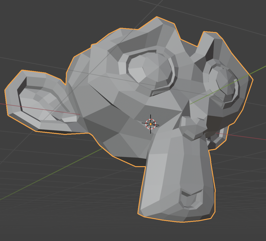
As a toy problem, we will aim for a nematic pattern on an initially spherical surfaces that reproduces “Suzanne”, a mesh model of a monkey’s head that is a common test case in the 3d software Blender:
Elastic energy
The elastic energy combines an in-plane and a bending contribution, using the framework of metric elasticity. The physical and “target” shape of an elastic sheet are described by two metric tensors, \(g\) and \(g_r\), which define the strain \(C = g_r^{-1} \cdot g\) (the identity in the stress-free state).
For the in-plane/stretch term, we use the neo-Hookean elastic energy of a thin sheet of thickness \(h\):
\[E_{\mathrm{nH}} = h \int dA \left[\frac{G_s}{2} \left(\frac{\mathrm{tr}\, C}{\sqrt{\det C}} - 2\right) + \frac{G_b}{2} \left(\sqrt{\det C} - 1\right)^2 \right]\] where \(G_s\) is the shear modulus and \(G_b\) the bulk modulus (area-stretch modulus). The elastic module implements a discrete version of this energy, by computing the metric \(g\) for each triangle from the 3D vertex positions. The integral becomes a sum over all triangles. The energy density diverges as a triangle is squashed (\(\det C \to 0\)), which makes it robust for large deformations. (The elastic module also provides the simpler St.-Venant-Kirchhoff energy, which is quadratic in the strain.)
Bending resistance is modeled using the 2nd fundamental form \(b\), which quantifies the extrinsic curvature of the surface: \[E_{\mathrm{B}} = G_f \int dA \, \mathrm{tr}\!\left[\left(g_r^{-1}(b-b_r)\right)^2 \right]\] where \(b_r\) is the target curvature and \(G_f \propto h^3\) is the flexural modulus: thin shells are much easier to bend than to stretch, as one may verify using a sheet of paper. In the code below, we set \(G_s = G_b = G_f = 1\) and \(h = 0.1\).
One way to generate target curvature is a bilayer with two different target metrics \(g_r^{t}, g_r^{b}\) (for top and bottom). Van Rees et al. showed that a bilayer is equivalent to a monolayer with
\[g_r = \frac{1}{2}(g_r^{t} + g_r^{b}), \quad b_r = \frac{3}{4h}(g_r^{t} - g_r^{b})\]
Sign convention: triangulax uses the “positive-convex” convention (a sphere with outward-pointing normals has \(b = +g\)), and the top layer is the side the face normals point to. With the \(+\) sign above, an expanding top layer creates positive target curvature.
Elastomers
Upon heating, a liquid crystal elastomer contracts along the local nematic director and expands orthogonal to it. In this model, this is captured by the reference metric. Initially, the reference metric equals the physical metric of the initial shape \(\mathcal{S}_0\), \(g_r = g_0\).
The change of target shape upon heating is described by a local strain tensor \[\Lambda(\theta) = R(\theta)^T \cdot \begin{pmatrix} \lambda & 0 \\ 0 & 1/\lambda \end{pmatrix} \cdot R(\theta) \] where \(R\) is a rotation matrix, \(\theta\) the local nematic angle, and \(\lambda\) the local expansion ratio along the director (by convention, \(\lambda < 1\) for a heated elastomer; choosing \(\lambda > 1\) is equivalent up to a rotation of the pattern). Since \(\det \Lambda = 1\), the actuation is locally area-preserving, which constrains the reachable target shapes. The reference metric deforms according to \[g_r = \Lambda^T \cdot g_0 \cdot \Lambda\]
Important — frames:
Our numerical implementation of the elastic energy follows Chen et al., 2018. The angles \(\theta^t, \theta^b\) are encoded per triangle, as an angle w.r.t. the first edge of the triangle. In the discrete elastic energies, the metric tensor and the curvature form are expressed in the basis of the triangle edges.
However, the rotation-matrix form of \(\Lambda\) holds in an orthonormal frame, but the discrete metrics of the elastic module are expressed in the (non-orthonormal) basis of the triangle edges. For a triangle with vertices \(a, b, c\), the edges are \(u = b-a\), \(v = c-a\), and the metric in the edge basis becomes \[g = \begin{pmatrix} u^2 & u\cdot v \\ v\cdot u & v^2 \end{pmatrix}\] We therefore use a change of basis \(B\) per triangle which moves from the \(u,v\) basis to an orthogonal basis. The rows of \(B\) are the edge vectors in the orthonormal frame with \(e_1=u / |u|\) and \(e_2 \perp e_1, |e_2| = 1\). In the \(B\)-basis, \(g_B = \mathbb{I}\) so that in the edge basis, \(g = B^T B\). The actuated reference metric in the edge basis is then \[g_r = B^T \cdot \Lambda(\theta)^T\Lambda(\theta) \cdot B, \qquad \Lambda^T\Lambda = \frac{\lambda^2 + \lambda^{-2}}{2}\,\mathbb{I} + \frac{\lambda^2 - \lambda^{-2}}{2}\begin{pmatrix} \cos 2\theta & \sin 2\theta \\ \sin 2\theta & -\cos 2\theta \end{pmatrix}\] The \(2\theta\)-dependence makes explicit that the director is a nematic (headless) degree of freedom: \(\theta\) and \(\theta + \pi\) are the same state.
For a bilayer elastomer, there are two local nematic orientations \(\theta^t, \theta^b\) that control the reference metrics of the top and bottom sheet. As we saw above, this is equivalent to changing the reference curvature of the sheet.
Inverse design
Our goal will be to program the local nematic orientations \(\theta^t, \theta^b\) so that an initially spherical mesh turns into a target shape. Given a nematic pattern \(\theta^t, \theta^b\), we simulate forward by minimizing the elastic energy. We can then compute a loss: the mean squared difference between the final vertex positions and the target. We can add extra terms to the loss, for example, encouraging smooth nematic fields. To solve the inverse design problem, we minimize the loss w.r.t. \(\theta^t, \theta^b\) using gradient-based optimization (the ADAM optimizer from optax). The gradient of the loss requires differentiating through the energy minimization \(\mathbf{v}^*(\boldsymbol{\theta}) = \arg\min E(\cdot\,; \boldsymbol{\theta})\): optimistix does this automatically via the implicit function theorem (no need to backpropagate through the iterations of the inner optimizer).
Since the elastic energy is invariant under rigid motions (translations and rotations), we first align the relaxed shape to the target with the differentiable Kabsch algorithm.
Targets
Before we turn to Suzanne, we will try this on less complex targets:
A teacher shape generated by the forward model itself (so we know a solution exists and can compare the recovered pattern to the ground truth).
A hand-designed deformed sphere (an ellipsoid).
import jax.numpy as jnp
import jaxjax.config.update("jax_enable_x64", True)
# note: keep jax_debug_nans off. the line searches inside the minimizers produce
# (safely handled) NaNs that would trigger false positives
jax.config.update("jax_debug_nans", False)from jaxtyping import Floatimport optimistix
import optaxfrom triangulax import geometry as geom
from triangulax import elastic
from triangulax import algorithms as algo
from triangulax import adjacency as adj
from triangulax import linops
from triangulax.triangular import TriMesh
from triangulax.mesh import HeMeshLoad mesh
We start with a very coarse unit sphere (42 vertices) so that experiments run in seconds. The sphere serves as both the initial condition and the rest configuration of the shell.
Throughout the tutorial, we consider meshes without boundary.
def load_sphere(name):
    """Loads, centers, and scales a sphere mesh from the tutorial_meshes/ directory."""
    mesh = TriMesh.read_obj(f"tutorial_meshes/{name}.obj", dim=3)
    vertices = mesh.vertices - mesh.vertices.mean(axis=0)
    vertices = jnp.asarray((vertices.T / np.linalg.norm(vertices, axis=1)).T)
    return vertices, HeMesh.from_triangles(vertices.shape[0], mesh.faces)

v0, hemesh = load_sphere("sphere") # use sphere_fine for a higher resolution mesh
metric_rest = elastic.get_metric(v0, hemesh)
b_rest = elastic.get_second_fundamental_form(v0, hemesh)

thickness, lam = 0.1, 1.1  # shell thickness h and nematic expansion ratio lambda
mod_shear = mod_bulk = 1.0  # shear, bulk, and flexural moduli G_s, G_b, G_f
mod_flex = 1 * thickness**2
hemesh
Warning: readOBJ() ignored non-comment line 3:
o IcosphereHeMesh(N_V=42, N_HE=240, N_F=80)Programming the reference metric with nematic directors
We now implement the actuation: per-face director angles \(\theta^t, \theta^b \mapsto\) reference metric \(g_r\) and reference curvature \(b_r\), following the formulas above.
def get_face_basis_from_metric(metric):
    """Per-face upper-triangular B with metric = B^T B (columns = edge vectors u, v
    in the orthonormal face frame e1 = u/|u|, e2 in-plane perpendicular)."""
    g00, g01 = metric[..., 0, 0], metric[..., 0, 1]
    det, sq = jnp.linalg.det(metric), jnp.sqrt(metric[..., 0, 0])
    zero = jnp.zeros_like(g00)
    return jnp.stack([jnp.stack([sq, g01 / sq], axis=-1),
                      jnp.stack([zero, jnp.sqrt(det) / sq], axis=-1)], axis=-2)


def get_nematic_metric(theta, lam, metric_rest):
    """Reference metric after nematic actuation: stretch lam along the director
    (angle theta from the first triangle edge), 1/lam orthogonal. Area-preserving.
    Final argument is the reference metric, which is used to compute the face basis
    in which the nematic metric is evaluated.
    """
    m = (lam**2 + lam**-2) / 2
    d = (lam**2 - lam**-2) / 2
    c2, s2 = jnp.cos(2 * theta), jnp.sin(2 * theta)
    Lam2 = jnp.stack([jnp.stack([m + d * c2, d * s2], axis=-1),
                      jnp.stack([d * s2, m - d * c2], axis=-1)], axis=-2)
    B = get_face_basis_from_metric(metric_rest)
    return jnp.einsum("...ji,...jk,...kl->...il", B, Lam2, B)


def get_bilayer_metric_and_curvature(theta_top, theta_bot, lam, metric_rest, b_rest, thickness):
    """Monolayer-equivalent (metric_ref, b_ref) for a bilayer with two director fields
    (van Rees et al. 2017). Top layer = side the face normals point to."""
    g_top = get_nematic_metric(theta_top, lam, metric_rest)
    g_bot = get_nematic_metric(theta_bot, lam, metric_rest)
    return (g_top + g_bot) / 2, b_rest + 3 / (4 * thickness) * (g_top - g_bot)
# tests: B^T B recovers the metric; lam=1 is the identity; actuation is area-preserving
B = get_face_basis_from_metric(metric_rest)
assert np.allclose(jnp.einsum("fji,fjk->fik", B, B), metric_rest)
assert np.allclose(get_nematic_metric(jnp.zeros(hemesh.n_faces), 1.0, metric_rest), metric_rest)
g_nem = get_nematic_metric(jnp.linspace(0, np.pi, hemesh.n_faces), lam, metric_rest)
assert np.allclose(jnp.linalg.det(g_nem), jnp.linalg.det(metric_rest))# to define smooth test patterns and to visualize directors, we need the orthonormal
# face frames (e1 along the first edge) in 3D world coordinates
def angle_from_global_direction(D, vertices, hemesh):
"""Per-face director angle (w.r.t. first edge) of a global 3D direction D
projected onto each face."""
e1, e2 = geom.get_face_tangent_basis(vertices, hemesh)
D = jnp.broadcast_to(D, e1.shape)
return jnp.arctan2(jnp.sum(D * e2, axis=-1), jnp.sum(D * e1, axis=-1))
def director_segments(theta, vertices, hemesh, scale=0.1, offset=0.0):
"""Line segments visualizing a per-face director field (for meshplot.add_lines)."""
e1, e2 = geom.get_face_tangent_basis(vertices, hemesh)
d = jnp.cos(theta)[:, None] * e1 + jnp.sin(theta)[:, None] * e2
centroids = geom.get_face_centroids(vertices, hemesh) + offset
return np.array(centroids - scale * d), np.array(centroids + scale * d)# example: the projection of the z-axis onto the sphere gives a smooth director
# field with defects at the poles (a nematic field on a sphere must have defects!)
theta_example = angle_from_global_direction(jnp.array([0., 0., 1.]), v0, hemesh)
p = meshplot.plot(np.array(v0), np.array(hemesh.faces), shading={"wireframe": True},
return_plot=True)
p.add_lines(*director_segments(theta_example, v0, hemesh), shading={"line_color": "red"})
p.save("tutorial_plots/06_director_field.html")Plot saved to file tutorial_plots/06_director_field.html.IFrame(src="tutorial_plots/06_director_field.html", width="100%", height=400) # for display in docs webpageThe forward model relaxes the shell to its energy minimum for given director fields. The total energy is the sum of the neo-Hookean in-plane energy \(h\,E_{\mathrm{nH}}\) and the bending energy \(G_f E_{\mathrm{B}}\) from above. We minimize with optimistix.NonlinearCG (for small meshes, a quasi-Newton method would also work).
def get_shell_energy(vertices, args):
    """Neo-Hookean shell energy: h * E_nH(G_s, G_b) + G_f * E_B, with E_B = sum_f A0_f tr(S^2),
    S = g_r^{-1} (b - b_r)."""
    hemesh, metric_ref, b_ref, thickness, mod_shear, mod_bulk, mod_flex = args
    E_s = elastic.get_neo_hookean_energy(vertices, (hemesh, metric_ref, mod_bulk, mod_shear))
    E_b = elastic.get_svk_bending_energy(vertices, (hemesh, metric_ref, b_ref, 0.0, mod_flex / 2))
    return thickness * E_s + mod_flex * E_b

solver = optimistix.NonlinearCG(rtol=1e-9, atol=1e-9)

def relax_shell(theta_top, theta_bot, v_init, hemesh, metric_rest, b_rest):
    """Minimize the shell energy for a given nematic pattern (differentiable)."""
    metric_ref, b_ref = get_bilayer_metric_and_curvature(theta_top, theta_bot, lam,
                                                         metric_rest, b_rest, thickness)
    sol = optimistix.minimise(get_shell_energy, solver, v_init,
                              (hemesh, metric_ref, b_ref, thickness, mod_shear, mod_bulk, mod_flex),
                              max_steps=4000, throw=False)
    return sol.value
# at lam = 1 (no actuation), the sphere is the exact rest state
metric_ref, b_ref = get_bilayer_metric_and_curvature(jnp.zeros(hemesh.n_faces),
jnp.zeros(hemesh.n_faces),
1.0, metric_rest, b_rest, thickness)
args = (hemesh, metric_ref, b_ref, thickness, mod_shear, mod_bulk, mod_flex)
assert np.isclose(get_shell_energy(v0, args), 0.0, atol=1e-12)
assert np.allclose(jax.grad(get_shell_energy)(v0, args), 0.0, atol=1e-10)What does a nematic pattern do?
Let’s actuate the sphere with a simple hand-picked teacher pattern where the top director is along the (projected) \(z\)-axis. If the bottom director is parallel to the top, the sphere is stretched along the \(z\) axis. Orthogonal directors in the two layers create a large metric mismatch, i.e. mainly a change of the reference curvature. This leads to buckling.
theta_teacher_top = angle_from_global_direction(jnp.array([0., 0., 1.]), v0, hemesh)

theta_teacher_bot = theta_teacher_top  # equal top and bottom directors
#theta_teacher_bot = theta_teacher_top + np.pi / 2 # orthogonal top and bottom directors

v_teacher = relax_shell(theta_teacher_top, theta_teacher_bot, v0, hemesh, metric_rest, b_rest)
displacement = jnp.linalg.norm(v_teacher - v0, axis=-1)
print(f"max displacement: {displacement.max():.3f} (sphere radius 1)")

p = meshplot.plot(np.array(v0), np.array(hemesh.faces), shading={"wireframe": True},
                  return_plot=True)
p.add_mesh(np.array(v_teacher) + np.array([2.5, 0, 0]), np.array(hemesh.faces),
           shading={"wireframe": True})
p.save("tutorial_plots/06_teacher_forward.html")
max displacement: 0.312 (sphere radius 1)Plot saved to file tutorial_plots/06_teacher_forward.html.IFrame(src="tutorial_plots/06_teacher_forward.html", width="100%", height=400)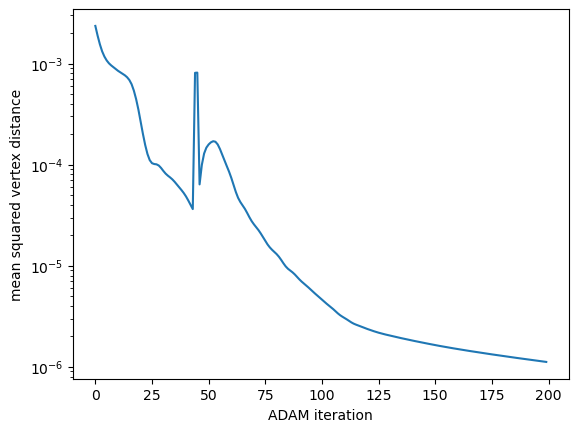
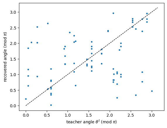
Inverse design 2: a hand-designed target
Now for a real design task: deform the sphere into a prescribed shape, in this case, an ellipsoid. Unlike the teacher target, an ellipsoid is generally not exactly reachable: the nematic actuation is locally area-preserving (\(\det \Lambda = 1\)) and the expansion ratio is fixed at \(\lambda\), so the design space is constrained. Gradient descent will find the best compromise.
v_ellipsoid = v0 * jnp.array([0.95, 0.95, 1.2])

loss = make_loss(v_ellipsoid, v0, hemesh, metric_rest, b_rest, reg=1e-3)
value_and_grad = jax.jit(jax.value_and_grad(loss, has_aux=True))

params = (jnp.zeros(hemesh.n_faces), jnp.zeros(hemesh.n_faces))
optimizer = optax.adam(learning_rate=0.1)
opt_state = optimizer.init(params)
history = []
for k in tqdm(range(200)):
    (L, fit), grads = value_and_grad(params)
    updates, opt_state = optimizer.update(grads, opt_state)
    params = optax.apply_updates(params, updates)
    history.append(fit)

v_designed = relax_shell(*params, v0, hemesh, metric_rest, b_rest)
err = jnp.linalg.norm(kabsch_align(v_designed, v_ellipsoid)[0] - v_ellipsoid, axis=-1)
print(f"fit {history[0]:.2e} -> {history[-1]:.2e}, max vertex error {err.max():.3f} "
      f"(target displacement scale {jnp.linalg.norm(v_ellipsoid - v0, axis=-1).max():.2f})")

plt.semilogy(history)
plt.xlabel("ADAM iteration"); plt.ylabel("mean squared vertex distance");
fit 6.09e-03 -> 5.15e-04, max vertex error 0.051 (target displacement scale 0.20)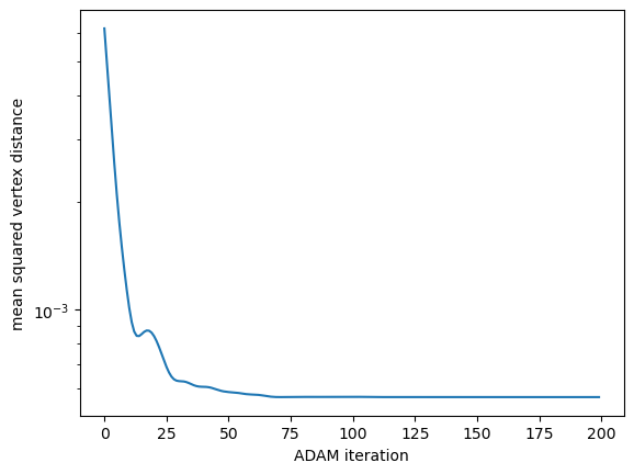
# left: designed shape (colored by vertex error, with the optimized top director
# field); right: the ellipsoid target
p = meshplot.plot(np.array(v_designed), np.array(hemesh.faces), np.array(err),
                  shading={"wireframe": True}, return_plot=True)
p.add_lines(*director_segments(params[0], v_designed, hemesh), shading={"line_color": "red"})
p.add_mesh(np.array(v_ellipsoid) + np.array([2.5, 0, 0]), np.array(hemesh.faces),
           shading={"wireframe": True})
p.save("tutorial_plots/06_ellipsoid_design.html")
Plot saved to file tutorial_plots/06_ellipsoid_design.html.IFrame(src="tutorial_plots/06_ellipsoid_design.html", width="100%", height=400)Scaling up
The same code runs on finer meshes, only slower: the inner elastic relaxation (and the linear solve in the implicit-differentiation backward pass) dominates, so on a 642-vertex sphere one ADAM iteration takes on the order of a second.
Warm-starting. An obvious acceleration idea is to “warm” start each relaxation from the equilibrium of the previous outer iteration. But this can lead to biased results: the elastic energy equilibrium reached from the warm-start is not necessarily the same as the one reached from the desired initial condition.
v0_fine, hemesh_fine = load_sphere("sphere_fine")
metric_rest_fine = elastic.get_metric(v0_fine, hemesh_fine)
b_rest_fine = elastic.get_second_fundamental_form(v0_fine, hemesh_fine)
v_target_fine = v0_fine * jnp.array([0.95, 0.95, 1.2])

loss = make_loss(v_target_fine, v0_fine, hemesh_fine, metric_rest_fine, b_rest_fine,
                 reg=1e-3)
value_and_grad = jax.jit(jax.value_and_grad(loss, has_aux=True))

params = (jnp.zeros(hemesh_fine.n_faces), jnp.zeros(hemesh_fine.n_faces))
optimizer = optax.adam(learning_rate=0.1)
opt_state = optimizer.init(params)
history_fine = []
for k in tqdm(range(100)):
    (L, fit), grads = value_and_grad(params)
    updates, opt_state = optimizer.update(grads, opt_state)
    params = optax.apply_updates(params, updates)
    history_fine.append(fit)

v_designed_fine = relax_shell(*params, v0_fine, hemesh_fine, metric_rest_fine, b_rest_fine)
err_fine = jnp.linalg.norm(kabsch_align(v_designed_fine, v_target_fine)[0] - v_target_fine,
                           axis=-1)
print(f"fit {history_fine[0]:.2e} -> {history_fine[-1]:.2e}, "
      f"max vertex error {err_fine.max():.3f}")
Warning: readOBJ() ignored non-comment line 4:
o Icospherefit 5.60e-03 -> 5.25e-04, max vertex error 0.051The final result shows a beautiful nematic pattern with two \(1/2\) defects on the poles of the ellipsoid.
p = meshplot.plot(np.array(v_designed_fine), np.array(hemesh_fine.faces), np.array(err_fine),
                  shading={"wireframe": False}, return_plot=True)
p.add_lines(*director_segments(params[0], v_designed_fine, hemesh_fine, scale=0.05),
            shading={"line_color": "red"})
p.add_mesh(np.array(v_target_fine) + np.array([2.5, 0, 0]), np.array(hemesh_fine.faces),
           shading={"wireframe": False})
p.save("tutorial_plots/06_ellipsoid_design_fine.html")
Plot saved to file tutorial_plots/06_ellipsoid_design_fine.html.IFrame(src="tutorial_plots/06_ellipsoid_design_fine.html", width="100%", height=400)Suzanne
Generating suzanne from the introduction from an initially spherical mesh will require a more complex pattern than an ellipsoid. We expect the outer optimizer to take longer (our Suzanne mesh has 1362 vertices, so a single relaxation takes several seconds).
Second, we need to rethink our loss function. If we start our simulation from the sphere_fine.obj mesh, we will have to compare meshes with different connectivity (simulation output vs Suzanne). Finding a good metric to compare meshes is challenging, and at the heart of active research in inverse design.
Therefore, we side-step the difficult mesh-mesh alignment problem. Instead, we turn the problem on its head. We start with a Suzanne mesh and attempt to find a nematic pattern that turns suzanne into a sphere (of arbitrary radius). For our loss function, we only need to evaluate whether the relaxed mesh vertices lie on a sphere. The position of the vertices in the final shape is now only constrained in the normal direction - we do not care where the vertices lie on the sphere. In addition, we add a penalty term that ensures that the mesh does not “get folded” (i.e., no two mesh points get mapped to the same point on the sphere). A folded configuration clearly is not a valid design! To do this, we penalize bending in the final configuration.
For the purpose of this tutorial, we will thus solve the simpler reverse problem of turning the Suzanne mesh into a sphere.
The mesh
Inverse design requires a well-conditioned underlying mesh: near-degenerate triangles make the discrete elastic energy ill-conditioned, and the outer optimization stalls or destroys the mesh. We therefore replace the Blender suzanne.obj mesh with a smoothed, cleaned-up version, suzanne_smooth.obj. The cell below verifies that it meets our requirements: closed, connected, manifold, outward-oriented, and with well-shaped triangles.
suzanne = TriMesh.read_obj("tutorial_meshes/suzanne_smooth.obj", dim=3) # suzanne_smooth
v0_suz = suzanne.vertices - suzanne.vertices.mean(axis=0)
v0_suz = jnp.asarray(v0_suz / np.sqrt((v0_suz**2).sum(axis=1).mean()))  # rms radius 1

v0_suz = v0_suz

hemesh_suz = HeMesh.from_triangles(v0_suz.shape[0], suzanne.faces)
metric_rest_suz = elastic.get_metric(v0_suz, hemesh_suz)
b_rest_suz = elastic.get_second_fundamental_form(v0_suz, hemesh_suz)

assert geom.get_volume(v0_suz, hemesh_suz) > 0  # outward normals
print(algo.get_mesh_quality_stats(v0_suz, hemesh_suz))
hemesh_suz
Warning: readOBJ() ignored non-comment line 3:
o suzanne_alpha_wrap_iso_remesh{'areas_min': 0.00057, 'areas_max': 0.00764, 'areas_cv': 0.22016, 'max_angle': 122.49484, 'min_angle': 21.59996, 'angles_std': 8.79166, 'n_degenerate': 0, 'n_total_faces': 2720}HeMesh(N_V=1362, N_HE=8160, N_F=2720)Sphericity loss
The “time-reversed” problem needs no mesh-to-mesh comparison at all: the loss only measures whether the relaxed vertices lie on some sphere. We use the relative radius variance,
\[\mathcal{L}_{\mathrm{sphere}}(\mathbf{v}) = \sum_i w_i \left(\frac{r_i}{\bar r} - 1\right)^2, \qquad r_i = |\mathbf{v}_i - \mathbf{c}|, \quad \bar r = \sum_i w_i r_i,\]
which is zero iff the vertices lie on any sphere (no alignment needed). The vertices are free to slide tangentially. The center \(\mathbf{c}\) and the mean radius are computed with barycentric-area weights \(w_i \propto A_i\), since the vertices need not be distributed uniformly on the sphere.
Avoiding fold-overs. During a first attempt with this loss, we found that the optimizer folds the protruding features (ears, snout) flat onto the sphere — not an acceptable elastomer design. To fix this, we penalize creases in the final configuration using the bending energy elastic.get_dihedral_bending_energy with flat target angles (\(\theta_e^0 = 0\)).
The optimization is also more challenging: the ADAM optimizer can overshoot in this rugged loss landscape, so we keep the best parameters seen. Note which iterate we keep: the penalties are an order of magnitude larger than the sphericity at the optimum, so the lowest-total-loss iterate is not the roundest one. We track the best sphericity among the iterates that stayed crease-free instead.
def get_nematic_curvature(theta, delta_theta, lam, metric_rest):
    d = (lam**2 - lam**-2) / 2
    c, s = jnp.cos(theta), jnp.sin(theta)
    R = jnp.stack([jnp.stack([c, -s], axis=-1),
                   jnp.stack([s, c], axis=-1)], axis=-2)
    eps = jnp.array([[0, 1], [1, 0]])
    Lam = d * delta_theta[:, None, None] * jnp.einsum("...ij,jk,...lk->...il", R, eps, R)
    B = get_face_basis_from_metric(metric_rest)
    return jnp.einsum("...ji,...jk,...kl->...il", B, Lam, B)


def get_bilayer_metric_and_curvature_alt(theta_mean, delta_theta, lam, metric_rest, b_rest, thickness):
    """Monolayer-equivalent (metric_ref, b_ref) for a bilayer with two director fields
    (van Rees et al. 2017). Top layer = side the face normals point to."""
    g_mean = get_nematic_metric(theta_mean, lam, metric_rest)
    b = get_nematic_curvature(theta_mean, delta_theta, lam, metric_rest)
    return g_mean, b_rest + 1 /thickness * b
# overall material parameters
thickness_suz = 0.1
lam_suz = 1.75 # Suzanne's drastic deformations require a larger expansion factor.
mod_shear = mod_bulk = 1
mod_flex = thickness_suz**2 * 1
solver = optimistix.NonlinearCG(rtol=1e-9, atol=1e-9)
def relax_suzanne(theta_top, theta_bot, v_init, lam=lam_suz):
"""Relax the Suzanne shell; lam_faces can be a scalar solver per-face array."""
metric_ref, b_ref = get_bilayer_metric_and_curvature(theta_top, theta_bot, lam,
metric_rest_suz, b_rest_suz,
thickness_suz)
sol = optimistix.minimise(get_shell_energy, solver, v_init,
(hemesh_suz, metric_ref, b_ref, thickness_suz,
mod_shear, mod_bulk, mod_flex),
max_steps=8000, throw=False)
return sol.value
def sphericity(v):
"""Area-weighted relative radius variance: 0 iff v lies on a sphere."""
areas = geom.get_barycentric_cell_areas(v, hemesh_suz)
w = areas / areas.sum()
center = (w[:, None] * v).sum(axis=0)
r = jnp.linalg.norm(v - center, axis=-1)
r_mean = (w * r).sum()
return (w * (r / r_mean - 1.0) ** 2).sum()
e1_suz, e2_suz = geom.get_face_tangent_basis(v0_suz, hemesh_suz)
f1_suz, f2_suz = hemesh_suz.heface, hemesh_suz.heface[hemesh_suz.twin]
def smoothness_suz(theta):
Q = compute_nematic_tensor(theta, e1_suz, e2_suz)
dQ_norm = ((Q[f1_suz] - Q[f2_suz]) ** 2).sum(axis=(-1, -2))
return dQ_norm.mean()
def loss_suzanne(params, reg_theta=1e-2, w_fold=1e-4):
theta_top, theta_bot = params
v_star = relax_suzanne(theta_top, theta_bot, v0_suz)
fit = sphericity(v_star)
fold = elastic.get_dihedral_bending_energy(v_star, (hemesh_suz, 0.0, 1.0))
penalty = (reg_theta * (smoothness_suz(theta_top) + smoothness_suz(theta_bot)) + w_fold * fold)
return fit + penalty, (fit, fold)
print(f"initial sphericity of Suzanne: {sphericity(v0_suz):.4f}")initial sphericity of Suzanne: 0.0322value_and_grad = jax.jit(jax.value_and_grad(loss_suzanne, has_aux=True))
params = (jnp.zeros(hemesh_suz.n_faces),
jnp.zeros(hemesh_suz.n_faces))
# to avoid instability, we need to decrease the learning rate of the optimizer over time
schedule = optax.piecewise_interpolate_schedule(
interpolate_type='linear',
init_value=0.5,
boundaries_and_scales={25: 0.2, 50: 0.2}) # decreases the lr by given factors at given times
optimizer = optax.adam(learning_rate=schedule)
opt_state = optimizer.init(params)
history_suz, history_suz_loss, best_fit, best_params = [], [], jnp.inf, params
# the penalties are an order of magnitude larger than the sphericity at the optimum, so the
# iterate with the lowest *total loss* is not the roundest one - track the best sphericity
# instead, among the iterates that stayed free of creases.
fold_max = 3 * elastic.get_dihedral_bending_energy(v0_suz, (hemesh_suz, 0.0, 1.0))
for k in tqdm(range(100)):
(L, (fit, fold)), grads = value_and_grad(params)
if fit < best_fit and fold < fold_max:
best_fit, best_params = fit, params # the iterate the loss was evaluated at
updates, opt_state = optimizer.update(grads, opt_state, params=params, value=L)
params = optax.apply_updates(params, updates)
history_suz.append(fit)
history_suz_loss.append(L)
print(f"iter {k:03d}: sphericity {fit:.4f}, penalty {L - fit:.2e}, loss {L:.4f}")iter 000: sphericity 0.0339, penalty 1.38e-01, loss 0.1722
iter 001: sphericity 0.0164, penalty 3.20e-01, loss 0.3363
iter 002: sphericity 0.0180, penalty 1.99e-01, loss 0.2167
iter 003: sphericity 0.0202, penalty 1.84e-01, loss 0.2046
iter 004: sphericity 0.0217, penalty 1.43e-01, loss 0.1644
iter 005: sphericity 0.0221, penalty 1.24e-01, loss 0.1458
iter 006: sphericity 0.0213, penalty 1.11e-01, loss 0.1323
iter 007: sphericity 0.0216, penalty 1.02e-01, loss 0.1234
iter 008: sphericity 0.0205, penalty 9.52e-02, loss 0.1157
iter 009: sphericity 0.0188, penalty 9.08e-02, loss 0.1096
iter 010: sphericity 0.0177, penalty 8.38e-02, loss 0.1015
iter 011: sphericity 0.0166, penalty 7.82e-02, loss 0.0947
iter 012: sphericity 0.0152, penalty 7.43e-02, loss 0.0895
iter 013: sphericity 0.0153, penalty 7.35e-02, loss 0.0887
iter 014: sphericity 0.0132, penalty 6.92e-02, loss 0.0824
iter 015: sphericity 0.0123, penalty 6.56e-02, loss 0.0780
iter 016: sphericity 0.0115, penalty 6.26e-02, loss 0.0741
iter 017: sphericity 0.0108, penalty 6.02e-02, loss 0.0710
iter 018: sphericity 0.0101, penalty 5.78e-02, loss 0.0679
iter 019: sphericity 0.0096, penalty 5.57e-02, loss 0.0653
iter 020: sphericity 0.0090, penalty 5.38e-02, loss 0.0628
iter 021: sphericity 0.0084, penalty 5.24e-02, loss 0.0608
iter 022: sphericity 0.0079, penalty 5.13e-02, loss 0.0592
iter 023: sphericity 0.0075, penalty 5.00e-02, loss 0.0575
iter 024: sphericity 0.0072, penalty 4.86e-02, loss 0.0559
iter 025: sphericity 0.0070, penalty 4.74e-02, loss 0.0544
iter 026: sphericity 0.0067, penalty 4.64e-02, loss 0.0531
iter 027: sphericity 0.0065, penalty 4.54e-02, loss 0.0519
iter 028: sphericity 0.0062, penalty 4.45e-02, loss 0.0508
iter 029: sphericity 0.0060, penalty 4.37e-02, loss 0.0497
iter 030: sphericity 0.0058, penalty 4.30e-02, loss 0.0488
iter 031: sphericity 0.0056, penalty 4.23e-02, loss 0.0479
iter 032: sphericity 0.0054, penalty 4.17e-02, loss 0.0471
iter 033: sphericity 0.0052, penalty 4.11e-02, loss 0.0463
iter 034: sphericity 0.0050, penalty 4.06e-02, loss 0.0456
iter 035: sphericity 0.0049, penalty 4.01e-02, loss 0.0449
iter 036: sphericity 0.0047, penalty 3.96e-02, loss 0.0443
iter 037: sphericity 0.0046, penalty 3.91e-02, loss 0.0437
iter 038: sphericity 0.0044, penalty 3.87e-02, loss 0.0431
iter 039: sphericity 0.0043, penalty 3.83e-02, loss 0.0426
iter 040: sphericity 0.0042, penalty 3.80e-02, loss 0.0422
iter 041: sphericity 0.0041, penalty 3.80e-02, loss 0.0421
iter 042: sphericity 0.0040, penalty 3.73e-02, loss 0.0413
iter 043: sphericity 0.0039, penalty 3.71e-02, loss 0.0410
iter 044: sphericity 0.0038, penalty 3.68e-02, loss 0.0406
iter 045: sphericity 0.0037, penalty 3.66e-02, loss 0.0403
iter 046: sphericity 0.0036, penalty 3.63e-02, loss 0.0400
iter 047: sphericity 0.0036, penalty 3.61e-02, loss 0.0397
iter 048: sphericity 0.0035, penalty 3.60e-02, loss 0.0395
iter 049: sphericity 0.0035, penalty 3.58e-02, loss 0.0393
iter 050: sphericity 0.0034, penalty 3.57e-02, loss 0.0391
iter 051: sphericity 0.0034, penalty 3.55e-02, loss 0.0389
iter 052: sphericity 0.0033, penalty 3.54e-02, loss 0.0387
iter 053: sphericity 0.0033, penalty 3.53e-02, loss 0.0386
iter 054: sphericity 0.0033, penalty 3.52e-02, loss 0.0384
iter 055: sphericity 0.0032, penalty 3.51e-02, loss 0.0383
iter 056: sphericity 0.0032, penalty 3.49e-02, loss 0.0381
iter 057: sphericity 0.0031, penalty 3.48e-02, loss 0.0380
iter 058: sphericity 0.0031, penalty 3.47e-02, loss 0.0378
iter 059: sphericity 0.0031, penalty 3.46e-02, loss 0.0377
iter 060: sphericity 0.0030, penalty 3.45e-02, loss 0.0375
iter 061: sphericity 0.0030, penalty 3.44e-02, loss 0.0374
iter 062: sphericity 0.0030, penalty 3.43e-02, loss 0.0372
iter 063: sphericity 0.0029, penalty 3.42e-02, loss 0.0371
iter 064: sphericity 0.0029, penalty 3.41e-02, loss 0.0369
iter 065: sphericity 0.0028, penalty 3.39e-02, loss 0.0368
iter 066: sphericity 0.0028, penalty 3.38e-02, loss 0.0366
iter 067: sphericity 0.0028, penalty 3.37e-02, loss 0.0365
iter 068: sphericity 0.0028, penalty 3.36e-02, loss 0.0364
iter 069: sphericity 0.0027, penalty 3.35e-02, loss 0.0362
iter 070: sphericity 0.0027, penalty 3.34e-02, loss 0.0361
iter 071: sphericity 0.0027, penalty 3.33e-02, loss 0.0359
iter 072: sphericity 0.0026, penalty 3.32e-02, loss 0.0358
iter 073: sphericity 0.0026, penalty 3.31e-02, loss 0.0357
iter 074: sphericity 0.0026, penalty 3.30e-02, loss 0.0355
iter 075: sphericity 0.0025, penalty 3.29e-02, loss 0.0354
iter 076: sphericity 0.0025, penalty 3.28e-02, loss 0.0353
iter 077: sphericity 0.0025, penalty 3.27e-02, loss 0.0351
iter 078: sphericity 0.0024, penalty 3.26e-02, loss 0.0350
iter 079: sphericity 0.0024, penalty 3.25e-02, loss 0.0349
iter 080: sphericity 0.0024, penalty 3.24e-02, loss 0.0347
iter 081: sphericity 0.0024, penalty 3.23e-02, loss 0.0346
iter 082: sphericity 0.0023, penalty 3.22e-02, loss 0.0345
iter 083: sphericity 0.0023, penalty 3.21e-02, loss 0.0344
iter 084: sphericity 0.0023, penalty 3.20e-02, loss 0.0342
iter 085: sphericity 0.0022, penalty 3.19e-02, loss 0.0341
iter 086: sphericity 0.0022, penalty 3.18e-02, loss 0.0340
iter 087: sphericity 0.0022, penalty 3.17e-02, loss 0.0339
iter 088: sphericity 0.0022, penalty 3.16e-02, loss 0.0337
iter 089: sphericity 0.0021, penalty 3.15e-02, loss 0.0336
iter 090: sphericity 0.0021, penalty 3.14e-02, loss 0.0335
iter 091: sphericity 0.0021, penalty 3.13e-02, loss 0.0334
iter 092: sphericity 0.0021, penalty 3.12e-02, loss 0.0332
iter 093: sphericity 0.0020, penalty 3.11e-02, loss 0.0331
iter 094: sphericity 0.0020, penalty 3.10e-02, loss 0.0330
iter 095: sphericity 0.0020, penalty 3.09e-02, loss 0.0329
iter 096: sphericity 0.0020, penalty 3.08e-02, loss 0.0328
iter 097: sphericity 0.0019, penalty 3.07e-02, loss 0.0327
iter 098: sphericity 0.0019, penalty 3.06e-02, loss 0.0325
iter 099: sphericity 0.0019, penalty 3.05e-02, loss 0.0324theta_top_suz, theta_bot_suz = best_params
v_sphered = relax_suzanne(theta_top_suz, theta_bot_suz, v0_suz)
r = jnp.linalg.norm(v_sphered - v_sphered.mean(axis=0), axis=-1)
r0 = jnp.linalg.norm(v0_suz - v0_suz.mean(axis=0), axis=-1)
dihedrals = jnp.abs(geom.get_dihedral_angles(v_sphered, hemesh_suz))
print(f"sphericity {history_suz[0]:.4f} -> {sphericity(v_sphered):.4f}, "
f"std(r)/mean(r): {r.std()/r.mean():.3f} (initially {r0.std()/r0.mean():.3f})")
print(f"largest dihedral angle: {jnp.degrees(dihedrals.max()):.0f} deg, "
f"edges folded beyond 90 deg: {int((dihedrals > jnp.pi/2).sum()) // 2}")
print(algo.get_mesh_quality_stats(v_sphered, hemesh_suz))
plt.semilogy(history_suz)
plt.semilogy(history_suz_loss)
plt.xlabel("ADAM iteration"); plt.ylabel("sphericity");sphericity 0.0339 -> 0.0019, std(r)/mean(r): 0.057 (initially 0.192)
largest dihedral angle: 30 deg, edges folded beyond 90 deg: 0
{'areas_min': 0.00075, 'areas_max': 0.01233, 'areas_cv': 0.33374, 'max_angle': 136.03523, 'min_angle': 12.92776, 'angles_std': 20.07503, 'n_degenerate': 0, 'n_total_faces': 2720}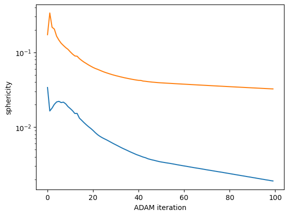
# the design is protocol-independent: quasi-statically ramping the actuation
# (slow heating, lambda(t) = 1 + t*(lambda - 1)) reaches the same final state

v_ramp = v0_suz
for t in [0.25, 0.5, 0.75, 1.0]:
    v_ramp = relax_suzanne(theta_top_suz, theta_bot_suz, v_ramp, lam=1.0 + t * (lam_suz - 1.0))
print(f"sphericity: direct relaxation {sphericity(v_sphered):.4f}, "
      f"quasi-static ramp {sphericity(v_ramp):.4f}")
sphericity: direct relaxation 0.0019, quasi-static ramp 0.0019# left: Suzanne colored by the optimized expansion factor lambda (per vertex,
# averaged from faces), with the top director field; right: the "spherized" result
view = np.diag([1, -1, -1])
p = meshplot.plot(np.array(v0_suz)@view, np.array(hemesh_suz.faces),
shading={"wireframe": False}, return_plot=True)
p.add_lines(*director_segments(theta_top_suz, v0_suz@view, hemesh_suz, scale=0.04),
shading={"line_color": "red"})
p.add_mesh(np.array(v_sphered)@view + np.array([3.0, 0, 0]), np.array(hemesh_suz.faces),
np.array(r / r.mean() - 1), shading={"wireframe": False})
p.save("tutorial_plots/06_suzanne_spherized_random_initial_cond_uniform_lam.html")Plot saved to file tutorial_plots/06_suzanne_spherized_random_initial_cond_uniform_lam.html.IFrame(src="tutorial_plots/06_suzanne_spherized_random_initial_cond_uniform_lam.html",
width="100%", height=400)The design flattens Suzanne substantially — the relative radius spread drops from 0.19 to about 0.06 — and, thanks to the fold penalty, the mesh has no creases and no degenerate triangles. Unfortunately, the snout and the ears are not quite flat. This indicates that the target shape lies beyond what can be reached for the possible internal strains.