JAX-compatible triangular meshes and triangular-mesh-based biophysics simulations
Overview
This Python package provides data-structures for triangular meshes, a geometry processing toolkit based on discrete differential geometry, and tools for simulating membranes, thin shells, and tissue sheets. The code is implemented in JAX and fully compatible with automatic differentiation and just-in-time compilation.
Many physical and biological systems, like foams, membranes, elastic shells, or tissue sheets, can be mathematically described as 2D surfaces. These surfaces can host complex dynamics, like reaction-diffusion systems, and undergo drastic deformations. Triangulax simulates the systems by discretizing continuous surfaces into triangular meshes. The library can also be applied to inherently discrete systems, like vertex models for epithelial tissues. It combines two features. First, discrete differential geometry provides coordinate-free discretization, which allow simulating strongly deforming surfaces. Second, the library is built on the machine-learning framework JAX, so mesh-based energies and entire simulations can be differentiated automatically. This simplifies multi-physics simulations by computing forces automatically and allows fitting model parameters to experimental data or design objectives. We implement an algorithm to preserve mesh quality in strongly deforming surfaces and apply it to a model of membrane mechanics coupled to an on-membrane concentration field. The discretizations have been validated against exact solutions and existing software. This repository includes tutorials on membrane mechanics, vertex models, and inverse design using machine-learning tools.
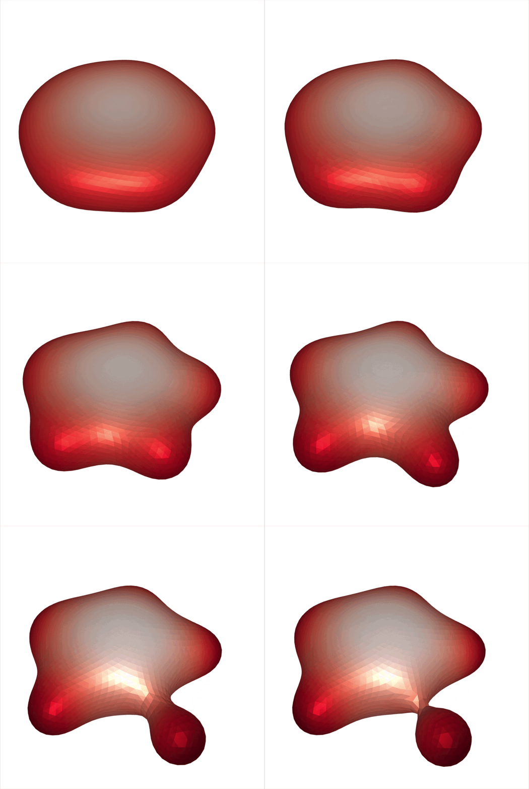
Simulation of membrane mechanics coupled to a concentration pattern (red), based on Leibler, J. Phys. France, 1986
Design
triangulax is designed for modularity and flexibility. The library includes a suite of geometry processing tools based on discrete differential geometry (Voronoi duals, curvatures, Laplace operator, …) and represents surfaces as half-edge meshes.
Automatic differentiation and just-in-time compilation with JAX
The main feature of triangulax is (forward- and reverse-mode) automatic differentiation to compute of derivatives of any mesh-based function. triangulaxuses JAX, a “Python library for accelerator-oriented array computation and program transformation, designed for high-performance numerical computing and large-scale machine learning.” Most triangulax functions are compatible with JAX’s just-in-time (JIT) compilation. JIT provides high performance in Python (rather than C++) and allows running on GPUs.
To simulate dynamics or minimize energies, triangulax integrates with JAX ecosystem libraries like optimistix (optimization) and diffrax (ODE integration), creating end-to-end differentiable simulations.
Prerequisites: triangulax assumes familiarity with triangular meshes (tutorial 0), and basic JAX usage (tutorial 1)
Use cases
Triangular meshes are ubiquitous in computer graphics and in scientific computing. Examples in soft-matter and biophysics include:
Reaction-diffusion systems on 3D curved surfaces (tutorial 4)
Mechanics of membranes and thin elastic shells in 3D (tutorial 5)
These tasks revolve around a mesh-based “energy”. JAX automatically computes their gradients, making it easy to optimize energies or to simulate forces. For “multiphysics” simulations (e.g. reaction-diffusion systems on deforming surfaces), it suffices to specify the combined energy of the system - all forces and cross-terms are calculated automatically.
Inverse problems
Since triangulax is fully JAX-compatible, one can differentiate a simulation with respect to its parameters. This means one can apply gradient-based optimization to inverse problems (tutorial 2). Effectively, a simulation becomes a “neural network” which maps initial conditions to simulation results. The parameters of the simulation can be fitted to data, or optimized to find a mechanism that generates a desired shape.
Documentation
Documentation is hosted on GitHub pages. Jupyter notebooks tutorials are in the nbs/tutorials/ folder.
Installation instructions
The triangulax package is hosted on PyPI. Install it as follows:
(Recommended) Initialize a virtual environment, for instance with conda:
simulation: Utilities for time-dependent simulations and checkpointing
Minimal example
import jaximport jax.numpy as jnpfrom triangulax import triangular, mesh, geometry# load example mesh and convert to half-edge meshvertices, faces = triangular.read_obj("test_meshes/disk.obj", dim=2)hemesh = mesh.HeMesh.from_triangles(vertices.shape[0], faces)# with the half-edge mesh, you can carry out various operations, for example# compute the coordination number by summing incoming half-edges per vertexcoord_number = jnp.zeros(hemesh.n_vertices)coord_number = coord_number.at[hemesh.dest].add(jnp.ones(hemesh.n_hes))print("Mean coordination number:", coord_number.mean())# Let's define a simple geometric function and compute its gradient with JAXdef mean_voronoi_area(vertices: jax.Array, hemesh: mesh.HeMesh) -> jax.Array:"""Compute the mean Voronoi area per vertex.""" voronoi_areas = geometry.get_voronoi_areas(vertices, hemesh)return jnp.mean(voronoi_areas)value, gradient = jax.value_and_grad(mean_voronoi_area)(vertices, hemesh)print("Mean gradient norm:", jnp.linalg.norm(gradient, axis=1).mean())
Warning: readOBJ() ignored non-comment line 3:
  o flat_tri_ecmc
Mean coordination number: 5.40458
Mean gradient norm: 0.0003638338
See also
libigl Geometry processing library with Python bindings. You can use libigl functions on triangulax meshes via the .faces attribute
This package is developed based on Jupyter notebooks, which are converted into python modules using nbdev. Details are in .github/copilot-instructions.md.