import numpy as np
import matplotlib.pyplot as plt

import copy

from tqdm.notebook import tqdmTutorial: Mesh optimization and inverse problems
Let’s start with a simple test case to see triangulax in action. The goal is to move the vertices \(\mathbf{v}_i\) of a triangulation so that all triangle edge lengths are as close to some \(\ell_0\) as possible. We specify a pseudo-energy \(E(\{\mathbf{v}_i\}_i; \ell_0) =\sum_{ij} (|\mathbf{v}_i-\mathbf{v}_j| - \ell_0)^2\), and then minimize it using the gradients w.r.t the vertex positions, computed with JAX.
This defines the “forward pass” of our “dynamical” model. In a second step, we can meta-optimize over the model parameters (here \(\ell_0\)), to “learn” the dynamics that generate a desired shape.
import jax
import jax.numpy as jnpjax.config.update("jax_enable_x64", True)
jax.config.update("jax_debug_nans", True)
jax.config.update('jax_log_compiles', False)import diffrax
import equinox as eqx
# equinox has automated "filtering" of JAX-transforms. So we can work with objects which are not just pytrees of arrays
# (like neural networks) and appy jit, vmap etcfrom jaxtyping import Float
from typing import Tuple
import dataclasses
import functools# import previously defined modules
from triangulax import trigonometry as trg
from triangulax import mesh as msh
from triangulax.triangular import TriMesh
from triangulax.mesh import HeMesh, GeomMesh
from triangulax import geometry as geom
from triangulax import linops as linLoad example mesh
mesh = TriMesh.read_obj("tutorial_meshes/disk.obj")
hemesh = HeMesh.from_triangles(mesh.vertices.shape[0], mesh.faces)
geommesh = GeomMesh(*hemesh.n_items, vertices=mesh.vertices)

hemesh
Warning: readOBJ() ignored non-comment line 3:
o flat_tri_ecmcHeMesh(N_V=131, N_HE=708, N_F=224)fig = plt.figure(figsize=(4, 4))
plt.triplot(*geommesh.vertices.T, mesh.faces)
plt.axis("equal");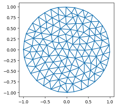
Forward pass - minimize energy
We write the energy_function using a GeomMesh as an argument, which serves as wrapper for the various arrays that describe mesh geometry and properties.
@jax.jit
def energy_function(geommesh: GeomMesh, hemesh: HeMesh, ell_0: float=1):
    edge_lengths = geom.get_he_length(geommesh.vertices, hemesh)
    edge_energy = jnp.mean((edge_lengths/ell_0-1)**2) # this way, term is "auto-normalized"
    # let's add a term for the triangle areas. Use the oriented area to penalize invalid mesh configurations
    a_0 = (np.sqrt(3)/4) * ell_0**2 # area of equilateral triangle
    tri_area = geom.get_oriented_triangle_areas(geommesh.vertices, hemesh)
    area_energy = jnp.mean((tri_area/a_0-1)**2)
    #jax.debug.print("E_l: {E_l}, E_a: {E_a}",  E_l=edge_energy, E_a=area_energy)
    # this is how you can print inside a JITed-function
    return edge_energy + area_energy
val, grad = jax.value_and_grad(energy_function)(geommesh, hemesh) # computing value and gradient of the energy
val, grad, grad.vertices.shape # the gradient is another GeomMesh. 1.60519339(Array(1.60519339, dtype=float64),
GeomMesh(D=2,N_V=131, N_HE=708, N_F=224),
(131, 2))connectivity_grad = jax.grad(energy_function, argnums=1, allow_int=True)(geommesh, hemesh)
# we can even compute the gradient w.r.t to the connectivity matrix. It is also a HeMesh
connectivity_grad, connectivity_grad.dest[0] # whatever that means(HeMesh(N_V=131, N_HE=708, N_F=224), np.void((b'',), dtype=[('float0', 'V')]))Energy optimization
Let’s follow the patterns described in the JAX tutorial to write a simulation time-stepping loop.
# time-stepping function
@jax.jit
def make_step(geommesh: GeomMesh, hemesh: HeMesh,
              current_time: Float[jax.Array, ""], next_time: Float[jax.Array, ""], ell_0: float = 1):
    loss, grad = jax.value_and_grad(energy_function)(geommesh, hemesh, ell_0=ell_0)
    updated_vertices = geommesh.vertices - (next_time-current_time)*grad.vertices
    geommesh = dataclasses.replace(geommesh, vertices=updated_vertices)
    return (geommesh, hemesh), loss # explicitly return the hemesh - may need to be updated by flips!
# simulation timesteps
step_size = 0.02
N_steps = 20000
timepoints = step_size * jnp.arange(N_steps)
# parameters of the energy
ell_0 = 0.5
# inital condition
init = ((geommesh, hemesh), timepoints[0])
# scanning function - applied at each time-step
def scan_function(carry, next_time: jax.Array):
(geommesh, hemesh), current_time = carry
(geommesh, hemesh), loss = make_step(geommesh, hemesh, current_time, next_time, ell_0=ell_0)
return ((geommesh, hemesh), next_time), loss # log the loss/energy# run the simulation
((geommesh_optimized, hemesh_optimized), _), loss = jax.lax.scan(scan_function, init, timepoints)fig = plt.figure(figsize=(4, 3))
plt.plot(loss)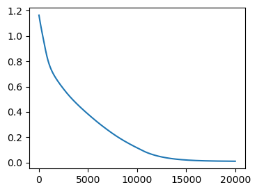
fig = plt.figure(figsize=(4, 4))
plt.triplot(*geommesh.vertices.T, hemesh.faces)
plt.triplot(*geommesh_optimized.vertices.T, hemesh_optimized.faces)
plt.axis("equal");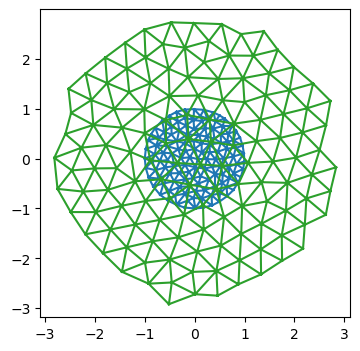
Using an ODE solver - diffrax
Above, we implemented “gradient descent” for the pseudo-energy, or, equivalently, a basic forward-Euler scheme for the ODE \(\partial_t \mathbf{v}_i = - \nabla_{\mathbf{v}_i} E\). For more complicated models, and to minimize coding effort, it makes sense to use a pre-made ODE solver instead. The diffrax library implements ODE and SDE solvers in JAX and is compatible with autodiff (you can differentiate through the solver), since it was designed for neural differential equations.
For “adiabatic” dynamics, which involve minimizing an energy at every time step, we can use the optimistix library.
The below is based on the Stepping through a solver tutorial in diffrax. The reason we want to step through the solver one-by-one is to carry out T1s (in future simulations).
# define the RHS for the ODE solver
@jax.jit
def vector_field(t, y, args):
    return jax.tree_util.tree_map(lambda x: -1*x, jax.grad(energy_function)(y, *args))
term = diffrax.ODETerm(vector_field)

# define time parameters and initial condition
dt = 0.05
t0 = 0.0
t1 = 1000.0
step_times = jnp.arange(t0, t1, dt)

y0 = geommesh
args = (hemesh, ell_0)

# initialize the solver
solver = diffrax.Tsit5()
y = y0
state = solver.init(term, t0, t0+dt, y0, args)
# scan through the solve
def scan_fun(carry, t):
state, y, tprev = carry
y, _, _, state, _ = solver.step(term, tprev, t, y, args, state, made_jump=False)
return (state, y, t), None
init = (state, y0, t0)
(state, y, t), _ = jax.lax.scan(scan_fun, init, step_times[1:])fig = plt.figure(figsize=(4, 4))
plt.triplot(*y0.vertices.T, hemesh.faces)
plt.triplot(*y.vertices.T, hemesh.faces)
plt.axis("equal");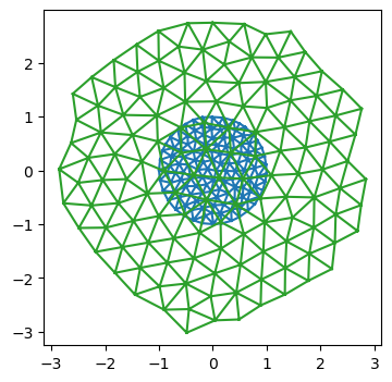
Backward pass - inverse problem
One use case for JAX is differentiating through a scientific simulation to optimize the simulation parameters towards some desired behavior. For example, we may wish to find a triangulation dynamics that creates some target shape.
As a toy example, let’s take the above “dynamics” which minimizes the pseudo-energy to make all triangles equilateral. It depends on the parameter \(\ell_0\). Relaxation of the pseudo-energy for some number of steps defines our “forward pass”. Let’s optimize \(\ell_0\) so that the mesh has some target size at the end of the energy relaxation (of course, this is a contrived problem, since we know the solution from the start).
First, we wrap our dynamical model as an eqx.Module, so we can optimize it just like a neural net.
class RelaxationDynamics(eqx.Module):
    ell_0: jax.Array
    step_size : float = eqx.field(static=True)
    N_steps : int = eqx.field(static=True)

    def __call__(self, initial_geommesh: GeomMesh, initial_hemesh: HeMesh) -> Tuple[GeomMesh, HeMesh]:
        init = ((initial_geommesh, initial_hemesh), 0)
        def scan_fun(i, carry):
            (geommesh, hemesh), _ = carry
            return make_step(geommesh, hemesh, ell_0=self.ell_0,
                             current_time=i*self.step_size, next_time=(i+1)*self.step_size)
        (geommesh_optimized, hemesh_optimized), _ = jax.lax.fori_loop(0, N_steps, scan_fun, init, unroll=None)
        return geommesh_optimized, hemesh_optimized
Define Meta-training loss
Now we need to define our meta-training loss. In this case, it’s just the deviation of the average edge length from the total. Note how the meta-loss is distinct from the pseudo-energy we minimize during the forward pass.
Let’s use the equinox library to handle our problem, in anticipation of more complex ones down the line.
# define the meta-loss

def meta_loss(model: RelaxationDynamics, initial_geommesh: GeomMesh, initial_hemesh: HeMesh,  meta_ell0: float) -> float:
    geommesh_optimized, hemesh_optimized = model(initial_geommesh, initial_hemesh)
    lengths = geom.get_he_length(geommesh_optimized.vertices,  hemesh_optimized)
    return jnp.mean((lengths/meta_ell0-1)**2)
# initialize the model, and test the meta loss
initial_ell0 = 0.4
meta_ell0 = 0.3
model_initial = RelaxationDynamics(ell_0=jnp.array([initial_ell0]), step_size=step_size, N_steps=N_steps)
model_initial(geommesh, hemesh), meta_loss(model_initial, geommesh, hemesh, meta_ell0=meta_ell0)((GeomMesh(D=2,N_V=131, N_HE=708, N_F=224),
HeMesh(N_V=131, N_HE=708, N_F=224)),
Array(0.13074658, dtype=float64))Batching
To evaluate the loss, we want to average over a bunch of initial conditions. These are analogous to batches in a normal ML problem.
## Let's create a bunch of meshes with different initial positions and see if we can batch over them using vmap

key = jax.random.key(0)
sigma = 0.02
N_batch = 3

batch_geom = []
batch_he = []
for i in range(N_batch):
    key, subkey = jax.random.split(key)
    random_noise = jax.random.normal(subkey, shape=geommesh.vertices.shape)
    batch_geom.append(dataclasses.replace(geommesh, vertices=geommesh.vertices+sigma*random_noise))
    batch_he.append(copy.copy(hemesh))

# we use a jax.tree.map to "push" the list axis into the underlying arrays.
# the result is a single mesh object with batch axes

batch_he_array = msh.tree_stack(batch_he)
batch_geom_array = msh.tree_stack(batch_geom)

batch_geom_array, batch_geom_array.vertices.shape
(GeomMesh(D=2,N_V=131, N_HE=708, N_F=224), (3, 131, 2))# We can apply the simulation and upack the results into a list
batch_geom_array_out, batch_he_array_out = jax.vmap(model_initial)(batch_geom_array, batch_he_array)
batch_geom_out = msh.tree_unstack(batch_geom_array_out)
batch_he_out = msh.tree_unstack(batch_he_array_out)# still works
i = 2
fig = plt.figure(figsize=(4, 4))
plt.triplot(*batch_geom[i].vertices.T, batch_he[i].faces)
plt.triplot(*batch_geom_out[i].vertices.T, batch_he_out[i].faces)
plt.axis("equal");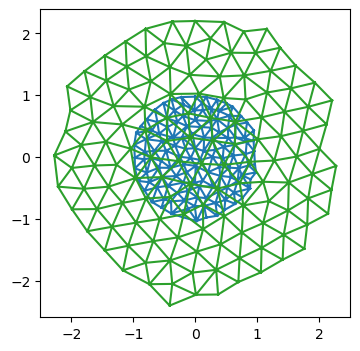
Compute the batched loss
# This is the right way to vmap the loss
jax.vmap(meta_loss, in_axes=(None, 0, 0, None))(model_initial, batch_geom_array, batch_he_array, 0.8)
Array([0.24862355, 0.24863542, 0.24863226], dtype=float64)# check against non-vmapped version. pretty similar, floating point errors likely at origin of differences
[meta_loss(model_initial, batch_geom_out[i], batch_he_out[i], 0.8) for i in range(3)][Array(0.24848931, dtype=float64),
Array(0.24848805, dtype=float64),
Array(0.2484898, dtype=float64)]Meta-optimization
Now we are in a position to “optimize” our model parameter ell_0. Based on equinox CNN tutorial.
def batched_meta_loss(model, batch_geom_array, batch_he_array, meta_ell0):
    return jnp.mean(jax.vmap(meta_loss, in_axes=(None, 0,0, None))(model, batch_geom_array, batch_he_array, meta_ell0))

batched_meta_loss_jit = jax.jit(batched_meta_loss)
# hyper-parameters for the outer learning step.
LEARNING_RATE = 1e-2
LEARNING_STEPS = 20
print_every = 2
step_size = 0.01
N_steps = 20000
META_ELL0 = 0.4
initial_ell0 = 0.2
model_initial = RelaxationDynamics(ell_0=jnp.array([initial_ell0]), step_size=step_size, N_steps=N_steps)loss, grads = eqx.filter_jit(eqx.filter_value_and_grad(batched_meta_loss))(model_initial,
batch_geom_array, batch_he_array, META_ELL0)
loss, grads, grads.ell_0(Array(0.24848878, dtype=float64),
RelaxationDynamics(ell_0=f64[1], step_size=0.01, N_steps=20000),
Array([-2.48070057], dtype=float64))Forward and reverse mode autodiff
Since we are differentiation w.r.t. a small number of parameters (just 1: \(\ell_0\)), we can use forward mode automatic differentiation for increased efficiency. This may be the case more generally: if we want to learn “translationally invariant” models, where the parameters for all cells are equal, the parameter count we want to differentiate by may be small. Forward mode autodiff is also somewhat more “forgiving” when it comes to control flow.
See: https://docs.jax.dev/en/latest/notebooks/autodiff_cookbook.html
@eqx.filter_jit
def outer_optimizer_step(model: RelaxationDynamics,
                         batch_geom: GeomMesh, batch_he: HeMesh) -> Tuple[RelaxationDynamics, float]:

    # compute loss and grad on batch
    loss, grads = eqx.filter_value_and_grad(batched_meta_loss)(model, batch_geom_array, batch_he_array, META_ELL0)
    updates = jax.tree.map(lambda g: None if g is None else -LEARNING_RATE * g, grads)
    model = eqx.apply_updates(model, updates)
    # grads is a PyTree with the same leaves as the trainable arrays of the model

    # same story, but using forward mode autodiff
    #loss, grads = eqx.filter_jvp(lambda model: batched_meta_loss(model, batch_geom_array, batch_he_array, META_ELL0),
    #                             primals=[model,], tangents=[model,])
    #grads = grads/model.ell_0 # we used the current model values as a tangent vector, so we need to normalize
    #model = dataclasses.replace(model, ell_0=model.ell_0-LEARNING_RATE*grads)

    return model, loss
model = model_initial
for step in tqdm(range(LEARNING_STEPS)): # in the future, could also iterate over the initial conditions/batches
model, loss = outer_optimizer_step(model, batch_geom_array, batch_he_array)
if (step % print_every) == 0:
print(f"Step: {step}, loss: {loss}, param: {model.ell_0}")
# 19s with forward mode vs 32s with reverse mode.Step: 0, loss: 0.24848877513396528, param: [0.22480701]
Step: 2, loss: 0.14704976288187882, param: [0.26531774]
Step: 4, loss: 0.08837946252729935, param: [0.29610925]
Step: 6, loss: 0.05458715535792712, param: [0.31944763]
Step: 8, loss: 0.03524215346058218, param: [0.33709312]
Step: 10, loss: 0.02417654272859851, param: [0.35045283]
Step: 12, loss: 0.01779509451762013, param: [0.36062556]
Step: 14, loss: 0.014058191845006396, param: [0.36843856]
Step: 16, loss: 0.01182824053575723, param: [0.37449757]
Step: 18, loss: 0.010471449413490624, param: [0.37924151]Looks good - the optimizer converges to the correct value of \(\ell_0\).
Next steps
Success: we can solve this (stupid) toy problem. Our JAX-compatible infrastructure for vertex models seems to work, and we can autodiff through a simulation. Next steps:
- Toy simulations with T1s
- More complex models - say, the area-perimeter vertex model
- Play around with neural ODEs and neural optimizers more generally.