from typing import Tuple

import dataclasses
import copy

import numpy as np

import matplotlib.pyplot as plt
import matplotlib as mpl

import jax
import jax.numpy as jnp

import diffrax
import lineax

from jaxtyping import Float, Bool, Int
from enum import IntEnum

import functoolsTutorial: Self-propelled Voronoi model
After the toy example of notebook 05, let’s implement a slightly more complicated model, the self-propelled Voronoi area-perimeter Voronoi (VAP) model of Bi et al., 2016. This 2D model comprises most of the ingredients we will see in more general tissue mechanics simulations, from a coding perspective.
In brief, in the VAP, cells are modeled as the Voronoi tesselation for a series of centroids \(\mathbf{v}_i\) (our triangulation vertices). Their overdamped dynamics comprises two terms: self-propulsion and relaxation of an elastic energy: \[\partial_t \mathbf{v}_i = -\nabla_{\mathbf{v}_i} E_{AP} + v_0 \hat{\mathbf{n}}_i\] For each cell \(i\), \(\hat{\mathbf{n}}_i\) is a unit vector (so we will represent it by an angle \(\theta_i\)) that determines the direction of motion. Units of time are chosen so that the coefficient of \(\nabla E_{AP}\) is \(1\). The energy is defined in terms of the Voronoi area \(a_i\) and Voronoi perimeter \(p_i\) of each cell: \[E_{AP} = \sum_i k_a(a_i-a_0)^2 + k_p(p_i-p_0)^2 \] where \(k_a, k_p\) are elastic constants, and \(a_0, p_0\) are the target area and perimeter. They define the “shape index” \(s_0= p_0/\sqrt{a_0}\). The key physics is that above a critical shape index \(s_0^*\), the model has a degenerate set of ground states, since for a large \(p_0\), there are many polygons with the given target area and perimeter (think floppy balloon).
The orientation \(\theta_i\) of each cell is also dynamic. It undergoes rotational diffusion: \[d\theta_i = D_\theta dW_{t, i} \] where \(dW_{t,i}\) is Brownian motion, independent for each cell \(i\), and \(D_\theta\) is the diffusion constant.
Numerics
The cell array connectivity will be represented by a HeMesh (see notebook 01). The geometry is fully described by the triangulation vertex positions, the Voronoi cell centroids. We also need a scalar vertex attribute for the angle \(\theta_i\). To calculate the energy \(E_{AP}\), we obtain Voronoi area and perimeter using the linops module. Boundary cells can be handled by “mirroring”, i.e., all corners count twice when computing the area/perimeter. Given the energy, JAX autodiff gives us the gradients. To time-evolve the mesh geometry, we can use diffrax, like in notebook 05. diffrax can also deal with SDEs, like the Langevin equation for cell angles.
Note This notebook is an example, and not meant to be numerically efficient!
jax.config.update("jax_enable_x64", True)
jax.config.update("jax_debug_nans", True)
jax.config.update("jax_log_compiles", False)
jax.config.update("jax_disable_jit", False)
from triangulax import trigonometry as trig
from triangulax.triangular import TriMesh
from triangulax import mesh as msh
from triangulax.mesh import HeMesh, GeomMesh
from triangulax.topology import flip_by_id
from triangulax import adjacency as adj
from triangulax import geometry as geomfrom importlib import reload
#reload(msh)
#reload(trig)Read in test data
mesh = TriMesh.read_obj("tutorial_meshes/disk.obj")
hemesh = HeMesh.from_triangles(mesh.vertices.shape[0], mesh.faces)
geommesh = GeomMesh(*hemesh.n_items, vertices=mesh.vertices)
geommesh = geom.set_voronoi_face_positions(geommesh, hemesh)

hemesh, geommesh
Warning: readOBJ() ignored non-comment line 3:
o flat_tri_ecmc(HeMesh(N_V=131, N_HE=708, N_F=224), GeomMesh(D=2,N_V=131, N_HE=708, N_F=224))fig, ax = plt.subplots(figsize=(4, 4))
ax.add_collection(msh.cellplot(hemesh, geommesh.face_positions,
cell_colors=np.array([0.7, 0.7, 0.9, 0.4]),
mpl_polygon_kwargs={"lw": 0.5, "ec": "k"}))
ax.set_aspect("equal")
ax.autoscale_view();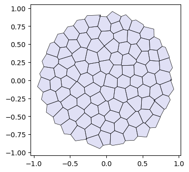
A note on periodic boundary conditions
The mesh we just loaded is a disk, and thus has a boundary. You may instead want to do simulations with periodic boundary conditions, i.e. simulate cells in a box with lengths \(\mathbf{L} = [L_x, L_y]\) where opposite sides are identified. The tools for this are implemented in the periodic module.
In triangulax, mesh connectivity and geometry are decoupled, so periodic boundary conditions are easy to implement. You need two ingredients:
- A triangulation whose connectivity has the desired periodicity (e.g. a triangulation of a torus).
There are different ways to generate a triangulation of the torus - one example is included in test_meshes/torus_2d.obj. Note: doing edge flips/T1 on this mesh will preserve its topology, no further bookkeeping needed. In particular, one does not need to keep track of any boundary vertices. There is no boundary! All triangulax tools related to the mesh connectivity (like the HeMesh class) can be used without modification.
- A distance function that takes into account the periodicity.
For a rectangular domain with lengths \(\mathbf{L} = [L_x, L_y]\), the displacement vector between two points \(\mathbf{r}_1, \mathbf{r}_2\) can be computed like this:
def displacement_periodic(r_1, r_2, L):
    d = r_2 – r_1
    return d – L*jnp.round(d/L)
This always gives the shortest displacement vector between the two points. With this distance function, you can compute edge lengths, angles, Voronoi duals, etc.
For a domain twisted/sheared along the \(x\)-axis by an amount \(s\) (i.e. a torus where \((x, y)\) and \((x + sL_x, y+L_y)\) are identified), the distance function becomes
def displacement_periodic_twisted(r_1, r_2, L, s):
    d = r_2 – r_1
    twist = s * L[0] * jnp.round(d[1] / L[1]) # compute the amount of twist
    d = d.at[0].set(d[0] + twist)
    return d – L*jnp.round(d/L)
Note: nothing prevents you from changing the shape of your domain, i.e. \(\mathbf{L}, s\) dynamically during your simulation! You can even take gradients with respect to them.
# this is an example of a 2d mesh with "periodic boundary conditions" - topologically, it is just a torus.
# you can see the faces that wrap around the boundary.

import igl

vertices, _, _, faces, _, _ = igl.readOBJ("tutorial_meshes/torus_2d.obj")

plt.triplot(vertices[:,0], vertices[:,1], faces, lw=0.5, color="k")
plt.axis("equal")
(np.float64(-0.028125350000000004),
np.float64(1.04895835),
np.float64(0.03749965),
np.float64(1.04583335))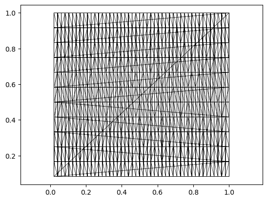
igl.boundary_loop_all(faces) # the mesh has no boundary[]Voronoi geometry and area-perimeter energy
def get_voronoi_perimeters(vertices: Float[jax.Array, "n_vertices dim"], hemesh: msh.HeMesh) -> Float[jax.Array, " n_vertices"]:
    """Compute Voronoi perimeters for each vertex."""
    voronoi_lengths = geom.get_voronoi_edge_lengths(vertices, hemesh)
    cell_perims = adj.sum_he_to_vertex_incoming(hemesh, voronoi_lengths)
    return cell_perims
@jax.jit
def energy_ap(geommesh: GeomMesh, hemesh: HeMesh, a0: float, p0: float,
k_a: float = 1.0, k_p: float = 1.0, k_penalty: float=10) -> Float[jax.Array, ""]:
"""Area-perimeter energy for Voronoi cells.
Adds small penalty for triangles with negative area.
"""
cell_areas = geom.get_voronoi_areas(geommesh.vertices, hemesh)
cell_perimeters = get_voronoi_perimeters(geommesh.vertices, hemesh)
tri_areas = geom.get_oriented_triangle_areas(geommesh.vertices, hemesh)
# add a factor 2x for boundary vertices to account for missing triangles
cell_areas = jnp.where(hemesh.is_bdry, 2.0 * cell_areas, cell_areas)
cell_perimeters = jnp.where(hemesh.is_bdry, 2.0 * cell_perimeters, cell_perimeters)
a_min = 0.25*(a0/2)
penality = jnp.where(tri_areas < a_min, k_a * (tri_areas-a_min)**2, 0.0).mean()
return k_a*jnp.mean((cell_areas-a0)**2) + k_p * jnp.mean((cell_perimeters-p0)**2) + k_penalty*penalitycell_areas, cell_perimeters = (geom.get_voronoi_areas(geommesh.vertices, hemesh),
get_voronoi_perimeters(geommesh.vertices, hemesh))
a_mean, p_mean = (cell_areas[~hemesh.is_bdry].mean(), cell_perimeters[~hemesh.is_bdry].mean())
a_mean, p_mean, p_mean/np.sqrt(a_mean)--------------------------------------------------------------------------- NameError Traceback (most recent call last) Cell In[62], line 1 ----> 1 cell_areas, cell_perimeters = (geom.get_voronoi_areas(geommesh.vertices, hemesh), 2 get_voronoi_perimeters(geommesh.vertices, hemesh)) 4 a_mean, p_mean = (cell_areas[~hemesh.is_bdry].mean(), cell_perimeters[~hemesh.is_bdry].mean()) 5 a_mean, p_mean, p_mean/np.sqrt(a_mean) NameError: name 'geommesh' is not defined
energy_ap(geommesh, hemesh, a0=a_mean, p0=3*jnp.sqrt(a_mean))67.2 μs ± 397 ns per loop (mean ± std. dev. of 7 runs, 10,000 loops each)grad_energy = jax.jit(jax.grad(energy_ap))grad_energy(geommesh, hemesh, a0=a_mean, p0=3*jnp.sqrt(a_mean))177 μs ± 25.7 μs per loop (mean ± std. dev. of 7 runs, 1 loop each)Edge flips
After each time step, we need to check if the Voronoi edge lengths are below some threshold (the edge lengths can be computed on the fly), and, if so, we need to carry out edge flips. We need to ensure that we do not “re-flip” an edge. This can be done via “cool down” period (an edge flipped at step \(t\) cannot be flipped again for the next few steps).
@functools.partial(jax.jit, static_argnames=['cooldown_steps', 'max_flips'])
def apply_flips(geommesh: GeomMesh, hemesh: HeMesh, l_min_T1: float,
                cooldown_counter: Int[jax.Array, " n_hes"], cooldown_steps: int, max_flips: int = 10
                ) -> Tuple[HeMesh, Int[jax.Array, " n_hes"], Bool[jax.Array, " n_hes"],]:
    """
    Apply T1 edge flips with a per-edge cooldown.

    Flipps edges if they are shorter than l_min_T1. Bondary edges are not flipped.

    Only flips the max_flips shortest edges for efficiency.
    """
    edge_lengths = geom.get_voronoi_edge_lengths(geommesh.vertices, hemesh)

    allow_flip = (cooldown_counter == 0) & hemesh.is_unique & ~hemesh.is_bdry_edge
    edge_lengths = jnp.where(allow_flip, edge_lengths, 1000)
    ids = jnp.argsort(edge_lengths)[:max_flips]

    hemesh_next = flip_by_id(hemesh, ids, edge_lengths[ids] < l_min_T1)
    did_flip = (edge_lengths < l_min_T1) & (edge_lengths < edge_lengths[ids[-1]])
    cooldown_counter = jnp.where(did_flip, cooldown_steps, jnp.clip(cooldown_counter-1, 0))

    return hemesh_next, cooldown_counter, did_flip
hemesh_next, cooldown_counter, did_flip = apply_flips(geommesh, hemesh, l_min_T1=0.0,
cooldown_counter=0*jnp.ones(hemesh.n_hes),
cooldown_steps=1, max_flips=10)
did_flip.sum()Array(4, dtype=int64)_ = apply_flips(geommesh, hemesh, l_min_T1=0.0, cooldown_counter=jnp.zeros(hemesh.n_hes, dtype=jnp.int32), cooldown_steps=5,
max_flips=10)
# 100mus for single flip. 110 mus for 10 flips/tpt, 600 mus for scanning over and flipping all edges.97.6 μs ± 2.65 μs per loop (mean ± std. dev. of 7 runs, 10,000 loops each)Energy relaxation (no self-propulsion)
We first only relax the area–perimeter energy. We also need to allow for topological modifications of the mesh (T1s/edge flips). At every timestep, we check if any dual cell edge has negative length and flip it. To ensure we don’t flip the same edge multiple times, let’s use a cooldown period.
# energy parameters
a0 = a_mean
s0 = 3
p0 = s0*jnp.sqrt(a0)

# numerical parameters
step_size = 0.02
n_steps = 10000

cooldown_steps = 5
l_min_T1 = 0.0

cooldown_counter=0*jnp.ones(hemesh.n_hes)
# relax energy
@jax.jit
def relax_energy_step(geommesh: GeomMesh, hemesh: HeMesh,
a0: float, p0: float,
step_size: float = 0.01,
k_a: float = 1.0, k_p: float = 1.0) -> Tuple[GeomMesh, Float[jax.Array, ""]]:
loss, grad = jax.value_and_grad(energy_ap)(geommesh, hemesh, a0, p0, k_a, k_p)
updated_vertices = geommesh.vertices - step_size * grad.vertices
geommesh_updated = dataclasses.replace(geommesh, vertices=updated_vertices)
return geommesh_updated, loss
# package simulation time step into a function for jax.lax.scan
@jax.jit
def scan_fun(carry: Tuple[GeomMesh, HeMesh, Int[jax.Array, " n_steps"]], x: Float[jax.Array, " n_steps"]):
(geommesh_relaxed, hemesh_relaxed), cooldown_counter = carry
# step energy
geommesh_relaxed, loss = relax_energy_step(geommesh_relaxed, hemesh_relaxed, a0, p0, step_size=step_size)
# carry out T1s
hemesh_relaxed, cooldown_counter, to_flip = apply_flips(geommesh_relaxed, hemesh_relaxed, l_min_T1,
cooldown_counter, cooldown_steps)
#to_flip = jnp.zeros(2)
# return updated carry and metrics
log = jnp.array([loss, to_flip.sum()])
return ((geommesh_relaxed, hemesh_relaxed), cooldown_counter), logcooldown_counter = jnp.zeros(hemesh.n_hes)
sim_steps = jnp.arange(n_steps)
init = ((geommesh, hemesh), cooldown_counter)
((geommesh_relaxed, hemesh_relaxed), _), logs = jax.lax.scan(scan_fun, init, sim_steps)
energy, flip_count = logs.Tfig = plt.figure(figsize=(4, 3))
plt.plot(energy[::int(n_steps/1000)])
plt.xlabel("step")
plt.ylabel("energy")
# add a twin y axis that shows the cummulative number of flips
ax2 = plt.gca().twinx()
ax2.plot(jnp.cumsum(flip_count)[::int(n_steps/1000)], color="orange")
ax2.set_ylabel("cumulative flips", color="orange")
ax2.set_ylim([0,flip_count.sum()+1])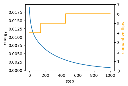
geommesh_relaxed = geom.set_voronoi_face_positions(geommesh_relaxed, hemesh_relaxed)

fig, ax = plt.subplots(figsize=(4, 4))
ax.add_collection(msh.cellplot(hemesh, geommesh.face_positions,
                               cell_colors=np.array([0.7, 0.7, 0.9, 0.2]),
                               mpl_polygon_kwargs={"lw": 0.5, "ec": "tab:blue"}))
ax.add_collection(msh.cellplot(hemesh_relaxed, geommesh_relaxed.face_positions,
                               cell_colors=np.array([0.9, 0.6, 0.6, 0.2]),
                               mpl_polygon_kwargs={"lw": 0.5, "ec": "tab:red"}))
ax.set_aspect("equal")
ax.autoscale_view();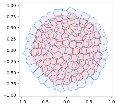
Overdamped dynamics with self-propulsion
omNext, let’s add the self-propulsion term. We initialize the angles \(\theta_i\) at random. We can store the angles as an extra vertex_attrib in our geommesh, using the functionality of the GeomMesh dataclass. We already have an IntEnum which we can use as keys to the vertex_attrib dictionary, like described in notebook 01.
In addition to incorporating the self-propulusion term \(\partial_t \mathbf{v}_i = -\nabla_{\mathbf{v}_i} E_{AP} + v_0\hat{\mathbf{n}}_i\), we need to do (stochastic) time steps for the angle orientation. Let’s do that with diffrax’s SDE solver, like in this tutorial. Let’s also implement the “pattern” for simulation loops with jax.lax.scan Note that the simulation can diverge if the self-propulsion term is too strong, due to effects at the boundaries. A more carefull handling of the boundaries (adding T1s on the boundaries, or using periodic BCs) is beyond the scope of this notebook.
Random numbers in JAX
JAX takes a different approach to random numbers (and hence the noise in our SDE) than numpy. The random numbers that will be used are specified by a key and will thus be reproducible across simulations. In particular, random numbers are no impediment to auto-differentiation; they are “frozen” when taking automatic derivatives.
## for this model, the simulation state becomes quite complex. Let's define a dataclass to hold it.

@jax.tree_util.register_dataclass
@dataclasses.dataclass
class SimState:
    geommesh: GeomMesh
    hemesh: HeMesh
    cooldown_counter: Int[jax.Array, " n_hes"]
    tprev: Float[jax.Array, ""]
    solver_state_sp: object
    solver_state_sde: object

## we also define a dataclass to hold logging information

@jax.tree_util.register_dataclass
@dataclasses.dataclass
class Log:
    geommesh: GeomMesh
    hemesh: HeMesh
    energy: Float[jax.Array, ""]
    n_flips: Int[jax.Array, ""]
# initialize orientations and store as a vertex attribute
class VertexAttribs(IntEnum):
SP_ORIENTATION = 1
key = jax.random.key(0)
theta0 = jax.random.uniform(key, shape=(hemesh.n_vertices,), minval=0.0, maxval=2*jnp.pi)
geommesh_sp = dataclasses.replace(geommesh,
vertex_attribs={VertexAttribs.SP_ORIENTATION: theta0})
hemesh_sp = copy.copy(hemesh)## set simulation parameters
# energy parameters
a0 = a_mean
s0 = 3
p0 = s0*jnp.sqrt(a0)
v0 = 0.005 # self-propulsion speed
ka = 1.0
kp = 1.0
# orientation dynamics parameters
diffusion_coeff_theta = 1.0
# timestepping parameters
step_size = 0.02
n_steps = 5000
cooldown_steps = 5
l_min_T1 = 0.0# check magnitude of the gradient forces vs the self-propulsion
grad0 = jax.grad(energy_ap)(geommesh_sp, hemesh, a0, p0, 1, 1).vertices
sp0 = v0*jnp.stack([jnp.cos(theta0), jnp.sin(theta0)], axis=-1)
jnp.linalg.norm(sp0, axis=-1).mean() / jnp.linalg.norm(grad0, axis=-1).mean()Array(1.5736791, dtype=float64)## define the ODE for vertex positions
@jax.jit
def ap_selfprop_vector_field(t: Float[jax.Array, ""],
y: GeomMesh,
args: Tuple[HeMesh, float, float, float, float, float]) -> GeomMesh:
"""RHS for overdamped area-perimeter dynamics with self-propulsion."""
hemesh, a0, p0, v0, k_a, k_p = args
theta = y.vertex_attribs[VertexAttribs.SP_ORIENTATION]
# combine energy gradient with self-propulsion
grad = jax.grad(energy_ap)(y, hemesh, a0, p0, k_a, k_p)
n_hat = jnp.stack([jnp.cos(theta), jnp.sin(theta)], axis=-1)
velocity = -grad.vertices + v0 * n_hat
# velocity = jnp.where(hemesh.is_bdry[:,None], 0, velocity)
# don't update the orientations here
zero_vertex_attribs = {key: jnp.zeros_like(val) for key, val in y.vertex_attribs.items()}
return dataclasses.replace(y, vertices=velocity, vertex_attribs=zero_vertex_attribs,)
term_sp = diffrax.ODETerm(ap_selfprop_vector_field)
## define the SDE and solver for orientation dynamics
key_sde = jax.random.key(0)
def diffusion(t, y, args):
return lineax.DiagonalLinearOperator(diffusion_coeff_theta*jnp.ones(hemesh_sp.n_vertices))
def drift(t, y, args):
return jnp.zeros(hemesh_sp.n_vertices)
brownian_motion = diffrax.VirtualBrownianTree(0, step_size*n_steps,
tol=1e-3, shape=(hemesh_sp.n_vertices,), key=key_sde)
term_sde = diffrax.MultiTerm(diffrax.ODETerm(drift), diffrax.ControlTerm(diffusion, brownian_motion))
## Define solvers
solver_sp = diffrax.Euler()
solver_sde = diffrax.EulerHeun()# initialize the ancillary variables (solver state, cooldown)
solver_state_sp = solver_sp.init(term_sp, 0, step_size, geommesh_sp, (hemesh_sp, a0, p0, v0, ka, kp))
solver_state_sde = solver_sde.init(term_sde, 0, step_size, geommesh_sp.vertex_attribs[VertexAttribs.SP_ORIENTATION], None)
timepoints = step_size * jnp.arange(n_steps)
init = SimState(geommesh=geommesh_sp, hemesh=hemesh_sp,
cooldown_counter= jnp.zeros(hemesh_sp.n_hes), tprev=timepoints[0],
solver_state_sp=solver_state_sp, solver_state_sde=solver_state_sde)# define the scan function - one step of the SDE + ODE coupled system
@jax.jit
def scan_fun(state: SimState, tnext: Float[jax.Array, ""],) -> tuple[SimState, Log]:
# time-step SDE for self-propulsion orientation
theta = state.geommesh.vertex_attribs[VertexAttribs.SP_ORIENTATION]
theta, _, _, solver_state_sde, _ = solver_sde.step(term_sde, state.tprev, tnext, theta,
None, state.solver_state_sde, made_jump=False)
# time-step ODE for vertex positions
args_sp = (state.hemesh, a0, p0, v0, ka, kp,)
geommesh, _, _, solver_state_sp, _ = solver_sp.step(term_sp, state.tprev, tnext, state.geommesh, args_sp,
state.solver_state_sp, made_jump=False,)
geommesh = dataclasses.replace(geommesh, vertex_attribs={VertexAttribs.SP_ORIENTATION: theta})
# T1 transitions for connectivity
hemesh, cooldown_counter, to_flip = apply_flips(geommesh, state.hemesh,l_min_T1,
state.cooldown_counter, cooldown_steps,)
# make measurements for log
energy = energy_ap(geommesh, hemesh, a0, p0, ka, kp)
n_flips=to_flip.sum()
log = Log(geommesh=geommesh, hemesh=hemesh,
energy=energy, n_flips=n_flips)
# package next state
next_state = SimState(geommesh=geommesh, hemesh=hemesh,
cooldown_counter=cooldown_counter, tprev=tnext,
solver_state_sp=solver_state_sp, solver_state_sde=solver_state_sde)
return next_state, logfinal_state, logs = jax.lax.scan(scan_fun, init, timepoints)Numerical efficiency
%%timeit shows that the simulation run above take about 1.7s. - The most expensive step is scanning for edge flips. You can probably accelerate the simulation a lot by checking only every \(n\) steps. - ODE solvers more complicated than diffrax.Euler perform worse, out of the box. You could likely use adaptive timestepping to greatly accelerate the simulation.
# Time stepping: scan advances (tprev -> tnext) for both theta and vertex dynamics.
final_state, logs = jax.lax.scan(scan_fun, init, timepoints)
1.71 s ± 7.39 ms per loop (mean ± std. dev. of 7 runs, 1 loop each)# Measurements logged at each step: geometry, connectivity, energy, and T1 flip counts.
geommesh_traj = msh.tree_unstack(logs.geommesh)
hemesh_traj = msh.tree_unstack(logs.hemesh)Visualize trajectory
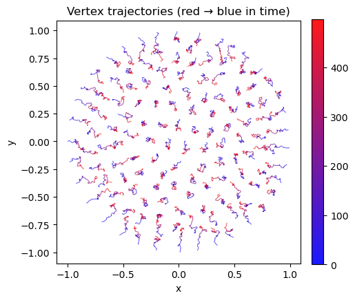
# total displacement - about 50% of a cell distance

mean_edge_len = geom.get_he_length(geommesh.vertices, hemesh).mean()

np.linalg.norm(geommesh_traj[0].vertices-geommesh_traj[-1].vertices, axis=-1).mean() / mean_edge_len
Array(0.54363885, dtype=float64)fig = plt.figure(figsize=(4, 3))
skip = int(np.ceil(n_steps/1000))
plt.plot(logs.energy[::skip])
plt.xlabel("step")
plt.ylabel("energy")
# add a twin y axis that shows the cummulative number of flips
ax2 = plt.gca().twinx()
ax2.plot(jnp.cumsum(logs.n_flips)[::skip], color="orange")
ax2.set_ylabel("cumulative flips", color="orange")
ax2.set_ylim([0,logs.n_flips.sum()+1])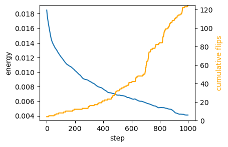
# angle dynamics are stochastic

fig = plt.figure(figsize=(4, 3))

cell_id = 50

plt.plot(logs.geommesh.vertex_attribs[VertexAttribs.SP_ORIENTATION][:, ::20])

plt.xlabel("step")
plt.ylabel("orientation")
Text(0, 0.5, 'orientation')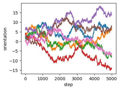
# plot initial and final mesh
fig, ax = plt.subplots(figsize=(4, 4))

geommesh_traj[-1] = geom.set_voronoi_face_positions(geommesh_traj[-1], hemesh_traj[-1])

ax.add_collection(msh.cellplot(hemesh_traj[0], geommesh_traj[0].face_positions,
                               cell_colors=np.array([0.7, 0.7, 0.9, 0.2]),
                               mpl_polygon_kwargs={"lw": 0.5, "ec": "tab:blue"}))
ax.add_collection(msh.cellplot(hemesh_traj[-1], geommesh_traj[-1].face_positions,
                               cell_colors=np.array([0.9, 0.6, 0.6, 0.2]),
                               mpl_polygon_kwargs={"lw": 0.5, "ec": "tab:red"}))


ax.set_aspect("equal")
ax.autoscale_view();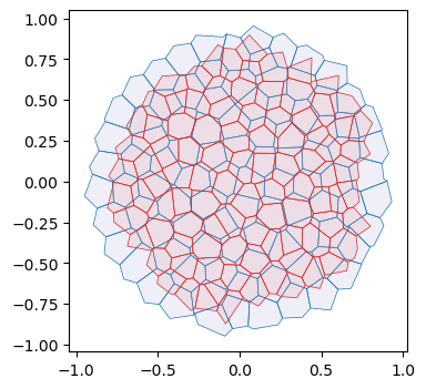
## plot trajectories of vertices (color = time: blue → red)

# logs.geommesh.vertices: (n_steps, n_vertices, 2), downsample in time
stride = 10
X = np.asarray(logs.geommesh.vertices)[::stride]
T = X.shape[0]

# Build line segments connecting consecutive time points for each vertex.
segments = np.stack([X[:-1], X[1:]], axis=2).reshape(-1, 2, 2)
t_idx = np.repeat(np.arange(T - 1), logs.geommesh.n_vertices)

cmap = mpl.colors.LinearSegmentedColormap.from_list("blue_to_red", ["blue", "red"])
norm = mpl.colors.Normalize(vmin=0, vmax=T - 2)

lc = mpl.collections.LineCollection(segments, cmap=cmap, norm=norm, linewidths=0.6, alpha=0.9)
lc.set_array(t_idx)

fig, ax = plt.subplots(figsize=(5, 5))
ax.add_collection(lc)
ax.set_aspect("equal")
ax.autoscale_view()
ax.set_title("Vertex trajectories (red → blue in time)")
ax.set_xlabel("x")
ax.set_ylabel("y")

cbar = fig.colorbar(lc, ax=ax, fraction=0.046, pad=0.04)