Using the half-edge mesh and the adjacency-like operators it defines, one can compute all sorts of geometric quantities of interest: edge lengths, cell areas, curvature in 3d, etc.
Discrete exterior calculus and discrete Hodge star
Triangle areas, cell areas, edge lengths, and dual edge lengths can be used to define the discrete version of the Hodge star operator used in discrete exterior calculus (DEC). See K. Crane’s lecture notes for an introduction to DEC.
Get lengths of half-edges (triangulation/primal edges).
Uses trigonometry.safe_norm, so a collapsed edge gives length 0 with a finite gradient rather than the NaN gradient of jnp.linalg.norm at the origin.
Intrinsic geometry from edge lengths
Almost every quantity in this notebook - triangle areas, corner angles, cotangent weights, the whole Voronoi dual - depends on the vertex positions only through the edge lengths \(\ell_{ij}\). Such quantities are called intrinsic: they are unchanged by any deformation that preserves edge lengths (bending a sheet of paper), and they are exactly the quantities an inhabitant of the surface could measure. The single-triangle formulas are in the trigonometry module (“Intrinsic geometry”); here we lift them to a whole mesh.
Each intrinsic function takes a per-half-edge array of edge lengths (as returned by get_he_length) instead of vertex positions, and is the implementation of the corresponding position-based function further below - get_voronoi_areas(vertices, hemesh), for instance, is get_voronoi_areas_intrinsic(get_he_length(vertices, hemesh), hemesh).
Working intrinsically has two payoffs:
Periodic (and Lees-Edwards) boundary conditions. Coordinate differences are meaningless across a periodic boundary, but edge lengths are not: compute them with a displacement function and hand them to the intrinsic functions. This is what the periodic module does - see notebook 05b. Working with the intrinsic geometry makes the tools from the geometry module easy to reuse.
Intrinsic triangulations and edge-length flows. Edge lengths can be treated as the primary degrees of freedom (e.g. optimizing a metric, or intrinsic Delaunay flips), with no embedding required at all.
Indexing convention. For half-edge he inside the triangle (he, nxt[he], prv[he]), the corner quantities (get_corner_angles_intrinsic, get_cotan_weights_per_he_intrinsic) refer to the corner oppositehe, i.e. at vertex dest[nxt[he]], matching the position-based functions below. The law of cosines then reads \(\cot\theta_{he} = (\ell_{nxt}^2 + \ell_{prv}^2 - \ell_{he}^2)/(4A)\). Boundary half-edges have no triangle and get 0.
Vectorized computation og cell areas, perimeters, etc for irregular meshes with gather/scatter
To compute, for instance, the cell area using the shoelace formula, you need to iterate around the faces adjacent to a vertex. This is not straightforward to vectorize because the number of adjacent faces per vertex can vary (there can be 5-, 6-, 7-sided cells etc.). One way to solve this is a scheme in which the lists of adjacent faces are “padded” in some manner, so that they are all the same length. This is cumbersome.
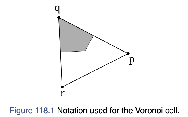
Instead, we split all “cell-based” quantities into contributions from “corners”, i.e., half-edges, like this:
To compute the total area, we can sum over all half-edges \((r,p)\) opposite to a vertex \(q\).
Robust Voronoi areas
The area assigned to a vertex by the Voronoi construction is an important quantity that shows up in many simulations and geometry operations. It can be computed according to the scheme above. We implement the “robust” version of the Voronoi area introduced by M Meyer, M Desbrun, P Schröder, A H Barr: “Discrete Differential-Geometry Operators for Triangulated 2-Manifolds”.
Angle of the corner opposite each half-edge, from edge lengths. 0 for boundary half-edges.
Uses theta = atan2(4A, l_nxt^2 + l_prv^2 - l_he^2) rather than arccos of the law of cosines, which stays accurate for angles near 0 and pi (see trigonometry.get_angles_from_lengths).
def get_triangle_areas_intrinsic( he_lengths:Float[Array, 'n_hes'], # Edge length per half-edge, e.g. from [`get_he_length`](https://nikolas-claussen.github.io/triangulax/src/geometric_quantities.html#get_he_length) or`periodic.get_periodic_he_lengths`. hemesh:HeMesh, # Half-edge mesh.)->Float[Array, 'n_faces']: # Unsigned area per face. Unlike [`get_oriented_triangle_areas`](https://nikolas-claussen.github.io/triangulax/src/geometric_quantities.html#get_oriented_triangle_areas), this cannotdetect inverted triangles - orientation isnot an intrinsic quantity.
Triangle areas from edge lengths (Heron’s formula).
Voronoi dual and curvature
The Voronoi dual (circumcentric dual) is intrinsic as well: dual edge lengths, cell areas and perimeters all follow from edge lengths and cotangent weights. The same holds for the Gaussian curvature - by Gauss’ theorema egregium it is determined by the metric alone, and its discrete version, the angle defect, only ever sees corner angles.
The geometric meaning of these quantities is discussed in the sections “Dual edge lengths and cell areas” and “Cell areas, perimeters, etc via corners” below; here we just give the intrinsic implementations, which the position-based functions there call.
Note what is not intrinsic, and therefore has no version here: anything that returns a position or an orientation - face centroids, circumcenter positions, normals, signed areas, and mean curvature. Edge lengths determine the shape of each triangle, not how the triangles are placed in space.
Angle defect 2*pi - sum(theta) from edge lengths, i.e. Gaussian curvature integrated over a vertex. 0 at boundary vertices, where it is not meaningful.
From Meyer et al. 2003, “Discrete Differential-Geometry Operators for Triangulated 2-Manifolds”
Uses the robust formula that handles obtuse triangles: - Non-obtuse triangle: use the Voronoi region area - Obtuse at vertex x: use area(T)/2 - Obtuse elsewhere: use area(T)/4
A corner is obtuse exactly when its cotangent is negative, so no angles are needed.
Compute oriented (signed) triangle areas in a mesh.
The shape of the result depends on the embedding dimension. In 3d it is the area-weighted face normal, of shape (n_faces, 3). In 2d it is a scalar signed area per face, of shape (n_faces,), positive for counter-clockwise triangles.
def get_triangle_orientations( vertices:Float[Array, 'n_vertices 2'], # Vertex positions in 2d. hemesh:HeMesh, # Half-edge mesh.)->Float[Array, 'n_faces']: # Orientation (+1/-1/0) per face.
Compute per-face orientation of a 2d mesh: +1, -1, or 0.
Returns +1 for counter-clockwise (positively oriented) triangles and -1 for clockwise (inverted) triangles. Exactly degenerate, zero-area triangles give 0. This is the 2d analogue of get_triangle_normals, and is useful to detect inverted triangles e.g. during mesh optimization.
def get_dihedral_angles( vertices:Float[Array, 'n_vertices 3'], # Vertex positions. hemesh:HeMesh, # Half-edge mesh.)->Float[Array, 'n_hes']: # Signed dihedral angle per half-edge (radians). 0 on boundary edges.
Get signed dihedral angles (angle between adjacent face normals).
Positive for convex edges, negative for concave. The sign is determined by the edge direction. Boundary edges have only one adjacent face, so no dihedral angle is defined there and 0 is returned.
Note: 3d meshes only.
Total volume and surface area
The volume \(V\) of a (closed) mesh can be discretized by breaking the mesh into tetrahedral pieces, one formed by each triangle plus the origin. For closed surfaces, the result is mathematically independent of the origin.
The gradient of the discrete volume w.r.t. vertex positions \(\mathbf{r}_i\) is \(\frac{dV}{d\mathbf{r}_i} = a_i \mathbf{n}_i\), where \(a_i\) is the vertex area (robust Voronoi), and \(\mathbf{n}_i\) the surface normal.
Signed volume of a closed triangulated surface (sums tetrahedra volumes relative to the origin [0., 0., 0.]).
The result is a mathematically meaningful volume only for a closed, consistently oriented mesh. For an open surface, the result will depend on the location of the origin.
The gradient of the volume w.r.t. vertex positions r_i is dV / dr_i = 1/3 * a_i * n_i, where a_i is the Voronoi area around vertex i, and n_i is the vertex normal. This is implemented via a custom JVP rule. Direct autodiff of the volume can lead to artifacts near topological defects in a mesh.
Dual edge lengths and cell areas (Voronoi construction)
The Voronoi dual of a triangular mesh is a cell tiling with one polygonal cell for every triangle vertex, one polygon edge per triangle edge, and one polygon corner per triangle. The corners of the Voronoi polygon are the triangles’ circumcenters. Therefore, the triangle and polygon edges are orthogonal. The Voronoi construction works in any dimension (since it is triangle-intrinsic).
Voronoi duals are important in discrete geometry and numerical simulations. For example, the Voronoi cell areas \(a_i\) are a way to assign areas to each vertex to discretize the area integral over a surface into a weighted sum over triangulation vertices, \(\int f dA \rightarrow \sum_i f_i a_i\)
Get lengths of dual/cell half-edges. Boundary edges get length 0.
Note the sibling get_oriented_dual_he_length uses 1 (not 0) for boundary edges, because a signed length of 0 is not distinguishable from a degenerate dual edge there.
a = get_dual_he_length(mesh.face_positions, hemesh)b = get_oriented_dual_he_length(mesh.vertices, mesh.face_positions, hemesh)jnp.allclose(a[~hemesh.is_bdry_edge], jnp.abs(b)[~hemesh.is_bdry_edge])
Array(True, dtype=bool)
# edges and dual edges should be orthogonal since we are using circumcentersface_positions = get_voronoi_face_positions(mesh.vertices, hemesh)edges = mesh.vertices[hemesh.orig]-mesh.vertices[hemesh.dest]dual_edges = (face_positions[hemesh.heface]-face_positions[hemesh.heface[hemesh.twin]])jnp.allclose(jnp.einsum('vi,vi->v', edges[~hemesh.is_bdry_edge], dual_edges[~hemesh.is_bdry_edge]), 0)
Array(True, dtype=bool)
# computing the signed edge length shows that there are some "flipped" edges.dual_length = get_oriented_dual_he_length(mesh.vertices, face_positions, hemesh)jnp.where((dual_length <-0.0) &~hemesh.is_bdry_edge )[0]
Corner angles, Gaussian curvature, cotangent weights, and Voronoi edge lengths/areas
These quantities are intrinsic: under the hood, they are computed from the edge lengths of the mesh (see “Intrinsic geometry from edge lengths” above).
# we can either compute the Voronoi-length of a dual edge directly, or from the face positionsvoronoi_edge_lengths = get_voronoi_edge_lengths(mesh.vertices, hemesh)dual_edge_length = get_oriented_dual_he_length(mesh.vertices, mesh.face_positions, hemesh)
Compute Voronoi cell area for each vertex by summing the areas in adjacent triangles (incoming half-edges)
Important: This function computes the exact Voronoi cell area (in any dimension), but can lead to numerical instabilities for very obtuse triangles. For use cases where the cell area serves as a tool (e.g. for discretizing the area integral), prefer get_voronoi_areas_robust.
Compute mixed Voronoi cell area (AMixed) for each vertex.
Uses the robust formula from Meyer et al. that handles obtuse triangles: - Non-obtuse triangle: use Voronoi region area - Obtuse at vertex x: use area(T)/2 - Obtuse elsewhere: use area(T)/4
See Fig 4 from M Meyer, M Desbrun, P Schröder, A H Barr: “Discrete Differential-Geometry Operators for Triangulated 2-Manifolds”
Voronoi perimeters (mean): 0.6346395879903053
Face centroids shape: (224, 2)
# for comparison, compute the areas by mesh traversalcell_areas = get_voronoi_areas(geommesh.vertices, hemesh)cell_areas = cell_areas.at[hemesh.is_bdry].set(0)cell_areas_iterative = _get_cell_areas_traversal(geommesh, hemesh)error = jnp.abs(cell_areas_iterative-cell_areas)print("Voronoi area max error:", error.max())
where the sum is over all triangles \(f\) neighboring vertex \(i\), and \(\phi_{i,f}\) is the angle in triangle \(f\) at vertex \(i\). We use the (robust) Voronoi cell area for the normalization \(a_i\) (so \(K_i\) is a density).
Angle defect represents the discrete Gaussian curvature integrated over a vertex.
Angle defect at boundary vertices is set to zero (since it is not meaningful there).
# Gaussian curvature should be 0 for a flat disk (interior vertices)K = get_gaussian_curvature(mesh.vertices, hemesh)print("Gaussian curvature (max interior):", jnp.abs(K[~hemesh.is_bdry]).max())
At a boundary vertex the angle defect is not a meaningful Gaussian curvature; the corresponding quantity is the geodesic curvature of the boundary curve, the exterior turning angle \(\kappa_g = \pi - \sum\theta\). Together with the interior angle defect it satisfies the discrete Gauss-Bonnet theorem.
Discrete geodesic curvature at boundary vertices: kappa_g = (pi - sum(theta)) / l.
Curvature is the exterior turning angle of the boundary curve. Interior vertices get 0, since geodesic curvature is only defined on the boundary.
The turning angle is divided by the dual boundary length at each vertex (half the sum of its two incident boundary edge lengths), giving a curvature density in 1/length.
Together with the angle defect it satisfies the discrete Gauss-Bonnet theorem: sum_interior (2*pi - sum theta) + sum_boundary (pi - sum theta) == 2*pi*chi, with chi the Euler characteristic (mesh.get_euler_characteristic).
Discrete curvature at boundary vertices: kappa_g = pi - sum(theta).
This is the exterior turning angle of the boundary curve. Interior vertices get 0, since geodesic curvature is only defined on the boundary.
Together with the angle defect it satisfies the discrete Gauss-Bonnet theorem: sum_interior (2*pi - sum theta) + sum_boundary (pi - sum theta) == 2*pi*chi, with chi the Euler characteristic (mesh.get_euler_characteristic).
# Gauss-Bonnet: sum of interior angle defects + boundary turning angles == 2*pi*chikappa_g = get_boundary_angle_defect(mesh.vertices, hemesh,)defect = jnp.where(hemesh.is_bdry, 0.0, 2*jnp.pi - get_angle_sum(mesh.vertices, hemesh))chi = msh.get_euler_characteristic(hemesh)total =float(defect.sum() + kappa_g.sum())print(f"Gauss-Bonnet on the disk: {total:.10f} vs 2*pi*chi = {2*jnp.pi*chi:.10f} (chi={chi})")assert jnp.allclose(total, 2*jnp.pi*chi, atol=1e-10)# interior vertices carry no geodesic curvatureassert jnp.all(kappa_g[~hemesh.is_bdry] ==0.0)# a flat convex polygon turns by 2*pi in totalassert jnp.allclose(kappa_g.sum(), 2*jnp.pi, atol=1e-10)# the normalized version is a density (1/length): it scales inversely with the meshk_dens = get_geodesic_curvature(mesh.vertices, hemesh)k_dens_scaled = get_geodesic_curvature(2*mesh.vertices, hemesh)assert jnp.allclose(k_dens[hemesh.is_bdry], 2*k_dens_scaled[hemesh.is_bdry], atol=1e-10)# and on a closed mesh it is identically zero_sph = TriMesh.read_obj("../test_meshes/sphere.obj", dim=3)_sph_h = msh.HeMesh.from_triangles(_sph.vertices.shape[0], _sph.faces)assert jnp.all(get_geodesic_curvature(_sph.vertices, _sph_h) ==0.0)
Gauss-Bonnet on the disk: 6.2831853072 vs 2*pi*chi = 6.2831853072 (chi=1)
Warning: readOBJ() ignored non-comment line 3:
  o Icosphere
Mean curvature
Two methods are provided for computing per-vertex mean curvature.
Steiner (dihedral angle) formula:\[H_i = \frac{1}{4ai} \sum_{j\sim i} \ell_{ij} \theta_{ij} \] where \(\theta_{ij}\) are the dihedral angles between adjacent triangles.
Cotangent Laplacian formula: using \(\Delta\mathbf{x} = 2H\mathbf{n}\), \[H_i = -\frac{\mathbf{n}_i \cdot (\Delta\mathbf{x})_i}{2 a_i}\] where and \(\Delta\) is the cotangent Laplacian.
In both cases, we use the (robust) Voronoi cell area for the normalization \(a_i\).
def get_mean_curvature_laplace( vertices:Float[Array, 'n_vertices 3'], # Vertex positions. hemesh:HeMesh, # Half-edge mesh. normalize:bool=True, # Whether to normalize by the robust Voronoi cell area. If False, returns themean curvature integrated over the Voronoi cell around each vertex.)->Float[Array, 'n_vertices']: # Per-vertex mean curvature (units: 1/length).
Compute mean curvature from the cotangent Laplacian: Δx = 2Hn.
The mean curvature of boundary vertices is set to 0.
Note: discrete curvature estimators can produce inaccurate results on poorly conditioned (non-Delaunay, highly anisotropic) meshes; consider algorithms.fix_delaunay and algorithms.get_mesh_quality_stats first. This method uses the cotangent Laplacian and is especially sensitive to non-Delaunay triangles (Laplacian loses positive-definiteness).
def get_mean_curvature_dihedral( vertices:Float[Array, 'n_vertices 3'], # Vertex positions. hemesh:HeMesh, # Half-edge mesh. normalize:bool=True, # Whether to normalize by the robust Voronoi cell area. If False, returns themean curvature integrated over the Voronoi cell around each vertex.)->Float[Array, 'n_vertices']: # Per-vertex mean curvature (units: 1/length).
Compute mean curvature of triangulated mesh using Steiner approximation: H_i = 1/(4 A_i) * sum_j * theta_ij * l_ij where theta_ij is the dihedral angle between faces adjacent to edge ij, l_ij is the length of edge ij, and A_i is the robust Voronoi cell area around vertex i.
The mean curvature of boundary vertices is set to 0.
Note: discrete curvature estimators can produce inaccurate results on poorly conditioned (non-Delaunay, highly anisotropic) meshes; consider algorithms.fix_delaunay and algorithms.get_mesh_quality_stats first.
# Test mean curvature on sphere and torus against libigl# --- Unit sphere ---v_sphere, f_sphere = igl.read_triangle_mesh("../test_meshes/sphere_fine.obj")v_sphere = v_sphere / np.linalg.norm(v_sphere, axis=-1, keepdims=True) # project to unit spherehemesh_sphere = msh.HeMesh.from_triangles(v_sphere.shape[0], f_sphere)v_sphere_jax = jnp.array(v_sphere)H_dihedral_sphere = get_mean_curvature_dihedral(v_sphere_jax, hemesh_sphere)H_laplace_sphere = get_mean_curvature_laplace(v_sphere_jax, hemesh_sphere)_, _, k1_s, k2_s, _ = igl.principal_curvature(v_sphere.astype(np.float64), f_sphere)H_igl_sphere = (k1_s + k2_s) /2print("=== Unit Sphere (H_true = 1.0) ===")print(f" igl: mean={np.mean(np.abs(H_igl_sphere)):.4f}, std={np.std(H_igl_sphere):.4f}")print(f" dihedral: mean={float(jnp.mean(jnp.abs(H_dihedral_sphere))):.4f}, std={float(jnp.std(H_dihedral_sphere)):.4f}")print(f" laplace: mean={float(jnp.mean(jnp.abs(H_laplace_sphere))):.4f}, std={float(jnp.std(H_laplace_sphere)):.4f}")
Warning: readOBJ() ignored non-comment line 4:
  o Icosphere
# --- Torus ---v_torus, f_torus = igl.read_triangle_mesh("../test_meshes/torus.obj")hemesh_torus = msh.HeMesh.from_triangles(v_torus.shape[0], f_torus)v_torus_jax = jnp.array(v_torus)H_dihedral_torus = get_mean_curvature_dihedral(v_torus_jax, hemesh_torus)H_laplace_torus = get_mean_curvature_laplace(v_torus_jax, hemesh_torus)_, _, k1_t, k2_t, _ = igl.principal_curvature(v_torus.astype(np.float64), f_torus)H_igl_torus = (k1_t + k2_t) /2print("\n=== Torus ===")print(f" igl: mean={np.mean(np.abs(H_igl_torus)):.4f}, range=[{H_igl_torus.min():.4f}, {H_igl_torus.max():.4f}]")print(f" dihedral: mean={float(jnp.mean(jnp.abs(H_dihedral_torus))):.4f}, range=[{float(H_dihedral_torus.min()):.4f}, {float(H_dihedral_torus.max()):.4f}]")print(f" laplace: mean={float(jnp.mean(jnp.abs(H_laplace_torus))):.4f}, range=[{float(H_laplace_torus.min()):.4f}, {float(H_laplace_torus.max()):.4f}]")# Correlation checkcorr_dihedral =float(jnp.corrcoef(jnp.array(H_igl_torus), H_dihedral_torus)[0, 1])corr_laplace =float(jnp.corrcoef(jnp.array(H_igl_torus), H_laplace_torus)[0, 1])print(f"\n Correlation with igl: dihedral={corr_dihedral:.4f}, laplace={corr_laplace:.4f}")# Note: the IGL quadratic fitting method does indeed give a different result than the Laplacian and dihedral methods (not a bug).# The difference between Laplace and dihedral methods is mostly due to the area normalization (voronoi vs barycentric).
Warning: readOBJ() ignored non-comment line 3:
  o Torus
# Regression test on a CURVED mesh WITH a boundary. Every 3d test above uses a closed# mesh and every boundary test uses the flat disk, where all dihedral angles are 0 --# so boundary bugs in the curvature path are invisible. Here the disk is bent onto a# cylinder of radius R, for which H = 1/(2R) and K = 0 exactly.R =2.0xy = mesh.vertices - mesh.vertices.mean(axis=0)v_cyl = jnp.stack([R*jnp.sin(xy[:, 0]/R), xy[:, 1], R*jnp.cos(xy[:, 0]/R)], axis=-1)interior =~hemesh.is_bdry# boundary edges have only one adjacent face, so no dihedral angle is defined there.# heface == -1 would silently index the LAST face instead.theta = get_dihedral_angles(v_cyl, hemesh)assert jnp.all(theta[hemesh.is_bdry_edge] ==0.0)H_dih = get_mean_curvature_dihedral(v_cyl, hemesh)H_lap = get_mean_curvature_laplace(v_cyl, hemesh)print(f"H interior: dihedral {H_dih[interior].mean():.4f}, laplace {H_lap[interior].mean():.4f} (exact {1/(2*R)})")# these estimators converge in a weak/measure sense: the mean over the patch is# accurate, while the pointwise error stagnates at irregular vertices.for H in [H_dih, H_lap]:assertabs(float(H[interior].mean()) -1/(2*R)) <1e-3assertfloat(jnp.median(jnp.abs(H[interior] -1/(2*R)))) <0.02# a cylinder is developable, so the angle defect vanishes up to discretization errordefect =2*jnp.pi - get_angle_sum(v_cyl, hemesh)assert jnp.abs(defect[interior]).max() <1e-2assertabs(float(defect[interior].sum())) <1e-2# curvature must be LOCAL: perturbing a vertex of the last face must not change# anything at a far-away boundary vertex.far =int(jnp.where(hemesh.is_bdry)[0][0])v_perturbed = v_cyl.at[int(hemesh.faces[-1][0])].add(jnp.array([0., 0., 0.3]))assert jnp.allclose(get_mean_curvature_dihedral(v_perturbed, hemesh)[far], H_dih[far], atol=1e-10)# 2d meshes have orientations rather than normalsorient = get_triangle_orientations(mesh.vertices, hemesh)assert jnp.all(jnp.abs(orient) ==1.0)assert jnp.all(get_triangle_orientations(mesh.vertices.at[:, 1].multiply(-1), hemesh) ==-orient)# gradients stay finite on a healthy meshfor fn in [get_mean_curvature_dihedral, get_mean_curvature_laplace, get_gaussian_curvature, get_voronoi_areas_robust, get_area]: g = jax.grad(lambda v: fn(v, hemesh).sum())(v_cyl)assert jnp.isfinite(g).all(), fn.__name__
H interior: dihedral 0.2501, laplace 0.2501 (exact 0.25)
Tangent spaces and parallel transport
This section defines tools to work with the tangent space of a surface, namely:
Bases for the tangent space at each vertex and face. We implement two bases:
Non-orthogonal local edge basis for faces. For a face with vertices \(a,b,c\), the basis is \(u=b-a, v=c-a\)
Local orthonormal bases in 3d coordinate-space for the tangent space at each vertex and face. For a face \(a,b,c\), this basis has vectors \(e_1 = (b-a)/|b-a|, \; e_2 \perp e_1\).
Parallel transport, which in the discrete setting means the rotation matrices that relate the local bases at adjacent triangles or vertices.
# load a 3D mesh for testing tangent space functionssphere = TriMesh.read_obj("../test_meshes/sphere.obj", dim=3)hemesh_s = msh.HeMesh.from_triangles(sphere.vertices.shape[0], sphere.faces)geommesh_s = msh.GeomMesh(sphere.vertices, sphere.face_positions)
Warning: readOBJ() ignored non-comment line 3:
  o Icosphere
Corner angles rescaled so they sum to 2π at interior vertices and π at boundary vertices.
Uses the same indexing convention as get_corner_angles: scaled_angles[he] is the rescaled angle at vertex dest[nxt[he]] (the vertex opposite halfedge he).
# test: scaled angles should sum to 2π at interior verticesscaled = get_corner_scaled_angles(geommesh_s.vertices, hemesh_s)scaled_sums = adj.sum_he_to_vertex_opposite(hemesh_s, scaled)assert jnp.allclose(scaled_sums[~hemesh_s.is_bdry], 2*jnp.pi, atol=1e-10)# for disk mesh (has boundary)scaled_disk = get_corner_scaled_angles(geommesh.vertices, hemesh)scaled_sums_disk = adj.sum_he_to_vertex_opposite(hemesh, scaled_disk)assert jnp.allclose(scaled_sums_disk[hemesh.is_bdry], jnp.pi, atol=1e-10)
Orthonormal tangent basis (basisX, basisY) in 3D world coordinates per face.
Convention: for a face with vertices (v0, v1, v2), basisX is (v1-v0)/|v1-v0| and basisY is the normalized in-plane component of (v2-v0), i.e. Gram-Schmidt. This makes (basisX, basisY, face_normal) right-handed, equivalently basisY = cross(normal, basisX). get_vertex_tangent_basis uses the same (right-handed) convention, so vectors can be moved between face and vertex frames consistently.
Note: works in 2d and 3d (no cross product is used).
Orthonormal tangent basis (basisX, basisY) in 3D world coordinates per vertex.
Convention: basisX is aligned with the vertex’ incident halfedge projected onto the vertex tangent plane, and basisY = cross(vertex_normal, basisX), so that (basisX, basisY, vertex_normal) is right-handed – the same handedness as get_face_tangent_basis.
Max bx·by: 6.497250925208836e-17
Max bx·n: 1.6653345369377348e-16
Parallel transport
To define parallel transport across an edge (between the tangent spaces of two adjacent triangles) or along an edge (between the tangent spaces of two adjacent vertices), we proceed as follows:
Find the coordinates of the shared edge vector \(\mathbf{e}_{ij} =\mathbf{v}_i-\mathbf{v}_j\) in the two local orthonormal bases, \((x, y)\) and \((x', y')\)
Compute the (minimal) rotation matrix that maps \((x, y)\) to \((x', y')\).
This defines two angles \(\phi_{ij}^v, \phi_{ij}^f\) for each half-edge, the discrete parallel transport map along (“v”) or across (“f”) the half edge.
def get_transport_across_halfedge( vertices:Float[Array, 'n_vertices dim'], # Vertex positions. hemesh:HeMesh, # Half-edge mesh.)->Float[Array, 'n_hes']: # Transport angle per halfedge (radians), in (-pi, pi]. 0 for boundary halfedges.
Rotation angle to transport a tangent vector from one face to the adjacent face across a halfedge.
Applying this rotation to a vector in the frame of heface[he] gives the same vector in the frame of heface[twin[he]]. For boundary half edges, this is set to 0 (no transport since there’s only one face).
The angle is signed, and consequently antisymmetric under the twin map: phi[twin[he]] == -phi[he]. Summing it around the one-ring of an interior vertex gives the holonomy, which equals minus the angle defect (modulo 2*pi).
# Parallel transport across an edge must be ANTIsymmetric under the twin map:# transporting frame f -> g and then g -> f must undo itself.transports = get_transport_across_halfedge(geommesh_s.vertices, hemesh_s)assert jnp.allclose(transports + transports[hemesh_s.twin], 0, atol=1e-10)# it must actually map the edge vector's coordinates from one face frame to the otherface_basis = get_face_tangent_basis(geommesh_s.vertices, hemesh_s)edge_vec = geommesh_s.vertices[hemesh_s.orig] - geommesh_s.vertices[hemesh_s.dest]coords_f = jnp.einsum('ivx, vx -> vi', face_basis[:, hemesh_s.heface], edge_vec)coords_g = jnp.einsum('ivx, vx -> vi', face_basis[:, hemesh_s.heface[hemesh_s.twin]], edge_vec)c, s = jnp.cos(transports), jnp.sin(transports)rot = jnp.stack([jnp.stack([c, -s], -1), jnp.stack([s, c], -1)], -2)assert jnp.allclose(jnp.einsum('vij,vj->vi', rot, coords_f), coords_g, atol=1e-10)# holonomy around a one-ring equals minus the angle defect (modulo 2*pi)defect =2* jnp.pi - get_angle_sum(geommesh_s.vertices, hemesh_s)wrap =lambda x: jnp.mod(x + jnp.pi, 2* jnp.pi) - jnp.pifor v in [0, 5, 20, 40]: holonomy = transports[jnp.array(hemesh_s.iterate_around_vertex(v))].sum()assert jnp.allclose(wrap(holonomy), wrap(-defect[v]), atol=1e-8)
def get_transport_along_halfedge( vertices:Float[Array, 'n_vertices dim'], # Vertex positions. hemesh:HeMesh, # Half-edge mesh.)->Float[Array, 'n_hes']: # Transport angle per halfedge (radians), in (-pi, pi]. 0 for boundary halfedges.
Rotation angle to transport a tangent vector from one vertex to the next vertex along a halfedge.
Applying this rotation to a vector in the frame of a vertex gives the same vector in the frame of the next vertex along the halfedge.
The angle is signed, and consequently antisymmetric under the twin map: phi[twin[he]] == -phi[he].
# Parallel transport along an edge must likewise be ANTIsymmetric under the twin map.transports = get_transport_along_halfedge(geommesh_s.vertices, hemesh_s)assert jnp.allclose(transports + transports[hemesh_s.twin], 0, atol=1e-10)# it must map the edge vector's coordinates from the orig frame to the dest framevertex_basis = get_vertex_tangent_basis(geommesh_s.vertices, hemesh_s)edge_vec = geommesh_s.vertices[hemesh_s.orig] - geommesh_s.vertices[hemesh_s.dest]coords_o = jnp.einsum('ivx, vx -> vi', vertex_basis[:, hemesh_s.orig], edge_vec)coords_d = jnp.einsum('ivx, vx -> vi', vertex_basis[:, hemesh_s.dest], edge_vec)c, s = jnp.cos(transports), jnp.sin(transports)rot = jnp.stack([jnp.stack([c, -s], -1), jnp.stack([s, c], -1)], -2)assert jnp.allclose(jnp.einsum('vij,vj->vi', rot, coords_o), coords_d, atol=1e-10)
 Source: