Convergence of the discrete differential-geometry operators

1. Test meshes

Each mesh is built from an isotropic remesh (plane_*, sphere_*, torus_* in refinement_tests/, at resolutions = edge length as % of the bounding-box diagonal, so 4 is coarsest and 0.25 finest) by:

Moving its vertices exactly onto the target surface (project to the sphere / torus apply a height deformation for the saddle and an anisotropic scaling for the ellipsoid), then
Flipping non-Delaunay edges with alg.fix_delaunay. This ensures mesh quality.

The five surfaces are the plane (\(K=H=0\)), a saddle \(z=\tfrac12(x^2-y^2)\) (a hyperbolic paraboloid, open), the unit sphere, an ellipsoid (sphere scaled by \((1,0.8,0.6)\)), and a torus (radii \(1,\,0.25\)). Delaunay-fixing is slow on the finest meshes, so the meshes are generated once and saved to refinement_tests/delaunay/; re-running skips meshes that already exist.

2. Analytical reference values

For a surface defined implicitly by as a level set \(F(x,y,z)=0\), the Gaussian and mean curvatures admit simple formulas Goldman 2005, which we evaluate by automatic differentiation

\[K=\frac{\nabla F^{\top}\operatorname{adj}(\mathbf H_F)\nabla F}{|\nabla F|^4},\qquad H=\frac{|\nabla F|^2\operatorname{tr}(\mathbf H_F)-\nabla F^{\top}\mathbf H_F\nabla F}{2|\nabla F|^3},\]

The sign is fixed so an outward-oriented sphere has \(H=+1/R\). The next cell checks this against the closed forms for the sphere (\(K=1/R^2\), \(H=1/R\)) and the ellipsoid.

def implicit_curvatures(F, x: Float[jax.Array, "3"]):
    """Gaussian K, mean H, and unit normal at a point x on the implicit surface F(x) = 0 (Goldman 2005)."""
    g = jax.grad(F)(x); Hess = jax.hessian(F)(x); gn2 = g @ g
    adj_H = jnp.array([
        [Hess[1,1]*Hess[2,2]-Hess[1,2]*Hess[2,1], Hess[0,2]*Hess[2,1]-Hess[0,1]*Hess[2,2], Hess[0,1]*Hess[1,2]-Hess[0,2]*Hess[1,1]],
        [Hess[1,2]*Hess[2,0]-Hess[1,0]*Hess[2,2], Hess[0,0]*Hess[2,2]-Hess[0,2]*Hess[2,0], Hess[0,2]*Hess[1,0]-Hess[0,0]*Hess[1,2]],
        [Hess[1,0]*Hess[2,1]-Hess[1,1]*Hess[2,0], Hess[0,1]*Hess[2,0]-Hess[0,0]*Hess[2,1], Hess[0,0]*Hess[1,1]-Hess[0,1]*Hess[1,0]]])
    K = (g @ adj_H @ g) / gn2**2
    H = (gn2*jnp.trace(Hess) - g @ Hess @ g) / (2 * gn2**1.5)
    return K, H, g / jnp.sqrt(gn2)

A_ELL, B_ELL, C_ELL = ELLIPSOID_AXES
IMPLICIT = {
    "sphere":    lambda x: x @ x - 1.0,
    "ellipsoid": lambda x: (x[0]/A_ELL)**2 + (x[1]/B_ELL)**2 + (x[2]/C_ELL)**2 - 1.0,
    "torus":     lambda x: (jnp.sqrt(x[0]**2 + x[1]**2) - TORUS_A)**2 + x[2]**2 - TORUS_C**2,
    "saddle":    lambda x: x[2] - SADDLE_AMPLITUDE * (x[0]**2 - x[1]**2),
    "plane":     lambda x: x[2],
}
def analytic_curvature(name, points):
    """Exact (K, H, unit normal) at each point, from the implicit representation."""
    return jax.vmap(lambda x: implicit_curvatures(IMPLICIT[name], x))(points)

# closed forms (Wikipedia) used only to validate the autodiff implementation
def sphere_KH(R=1.0): return 1/R**2, 1/R
def ellipsoid_KH(x, a=A_ELL, b=B_ELL, c=C_ELL):
    q = (x[...,0]/a**2)**2 + (x[...,1]/b**2)**2 + (x[...,2]/c**2)**2
    return 1/((a*b*c)**2*q**2), jnp.abs(x[...,0]**2+x[...,1]**2+x[...,2]**2-a**2-b**2-c**2)/(2*(a*b*c)**2*q**1.5)

key = jax.random.PRNGKey(0); p = jax.random.normal(key, (500, 3))
p_sphere = p/jnp.linalg.norm(p, axis=1, keepdims=True); p_ellip = p_sphere*jnp.array(ELLIPSOID_AXES)
for name, pts, (Kc, Hc) in [("sphere", p_sphere, sphere_KH()), ("ellipsoid", p_ellip, ellipsoid_KH(p_ellip))]:
    K, H, _ = analytic_curvature(name, pts)
    print(f"{name:10s} max|K-K_closed|={float(jnp.max(jnp.abs(K-Kc))):.1e}  max|H-H_closed|={float(jnp.max(jnp.abs(H-Hc))):.1e}")

sphere     max|K-K_closed|=4.4e-16  max|H-H_closed|=4.4e-16
ellipsoid  max|K-K_closed|=2.7e-15  max|H-H_closed|=1.8e-15

Error metric and reference integrals

For a quantity \(A\) we report the relative error, normalized by the surface-average magnitude, \(|A_{\rm exact}-A_{\rm disc}|/\overline{|A|}\) with \(\overline{|A|}=\int_S|A|\,dA/\int_S dA\). Both \(\overline{|A|}\) and the exact region integrals come from a fine parametric quadrature of each surface, which also fixes the sectors used later: 8 octants (ellipsoid, by coordinate sign), 8 poloidal bands (torus), and 8 angular sectors inside a disk of radius \(0.8\) (saddle).

3. Differential operators converge pointwise

We first check the two operators that do converge pointwise. The finite-element gradient is tested on the ambient-linear field \(u=a\cdot x\), whose exact surface gradient is the tangential projection \(a-(a\cdot n)\,n\) (with the smooth normal \(n\)). The area-normalised cotangent Laplace–Beltrami operator is tested on eigen/harmonic fields: on the sphere \(\Delta_S z=-2z\), on the plane \(\Delta(x^2+y^2)=4\). Errors are RMS over faces/vertices, normalised as above. Because the flat-mesh error is at machine precision while the curved-surface error is \(O(h)\), the \(y\)-axis is broken into two ranges.

/var/folders/vm/1jl6rjln6n9cjt54vsr9n4800000gr/T/ipykernel_24157/1943862201.py:64: UserWarning: This figure includes Axes that are not compatible with tight_layout, so results might be incorrect.
  plt.tight_layout(pad=0.1, w_pad=0.4, h_pad=0.1)
findfont: Font family 'normal' not found.
findfont: Font family ['normal'] not found. Falling back to DejaVu Sans.
findfont: Font family 'normal' not found.
findfont: Font family 'normal' not found.
findfont: Font family 'normal' not found.
findfont: Font family 'normal' not found.
findfont: Font family 'normal' not found.
findfont: Font family 'normal' not found.
findfont: Font family 'normal' not found.
findfont: Font family 'normal' not found.
findfont: Font family 'normal' not found.
findfont: Font family 'normal' not found.
findfont: Font family 'normal' not found.
findfont: Font family 'normal' not found.
findfont: Font family 'normal' not found.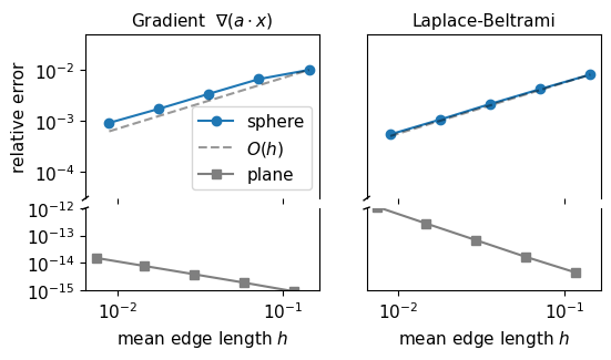

Both operators converge pointwise \(O(h)\) on the sphere and machine-exact on the plane (the P1 gradient of a linear field is exact on each triangle, and the cotan Laplacian is exact for the quadratic on a flat mesh).

4. Pointwise curvature: stable, but not convergent

The curvature estimators only converge in the weak sense. Below, the median pointwise error (bulk behavior) and the maximum pointwise error (worst vertex) are shown for \(K\) and \(H\) on the sphere and the ellipsoid. On the near-regular sphere the median converges like \(O(h^2)\), but on the ellipsoid, where the mesh is less regular, the median does not decrease. The maximum error stays bounded under refinement on both surfaces: the estimators are pointwise stable.

We also compare two discretizations of the mean curvature, using Laplace operator + Voronoi areas (get_mean_curvature_laplace, recommended), and dihedral angles + barycentric area.

Note that our implementation matches the libigl to machine precision – lack of pointwise convergence is a property of the discretisation, not a bug.

def get_mean_curvature_dihedral_barycentric(vertices, hemesh):
    H_dihedral = geom.get_mean_curvature_dihedral(vertices, hemesh, normalize=False)
    return H_dihedral / geom.get_barycentric_cell_areas(vertices, hemesh)

findfont: Font family 'normal' not found.
findfont: Font family 'normal' not found.
findfont: Font family 'normal' not found.
findfont: Font family 'normal' not found.
findfont: Font family 'normal' not found.
findfont: Font family 'normal' not found.
findfont: Font family 'normal' not found.
findfont: Font family 'normal' not found.
findfont: Font family 'normal' not found.
findfont: Font family 'normal' not found.
findfont: Font family 'normal' not found.
findfont: Font family 'normal' not found.
findfont: Font family 'normal' not found.
findfont: Font family 'normal' not found.
findfont: Font family 'normal' not found.
findfont: Font family 'normal' not found.
findfont: Font family 'normal' not found.
findfont: Font family 'normal' not found.
findfont: Font family 'normal' not found.
findfont: Font family 'normal' not found.
findfont: Font family 'normal' not found.
findfont: Font family 'normal' not found.
findfont: Font family 'normal' not found.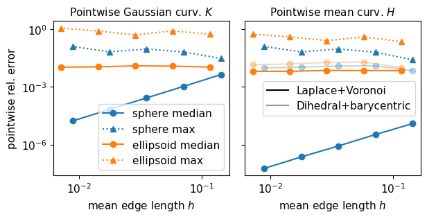

5. What convergence to expect

The behaviour above is exactly what the literature predicts. The angle-defect and cotangent curvature estimators are not guaranteed to converge pointwise on general meshes; they converge in an integrated / weak (“measure”) sense.

Gaussian curvature (angle defect). The defect \(2\pi-\sum_i\theta_i\) is the integral of \(K\) over the cell around a vertex (up to higher order); over a closed surface it is exactly \(2\pi\chi\) (Gauss–Bonnet). Divided by the cell area it converges pointwise only for meshes with special regularity properties. However, Cohen-Steiner & Morvan prove that discrete curvature measures converge over any fixed region, linearly \(O(h)\) in the sampling density.
Mean curvature (cotangent). The cotan Laplacian converges to its smooth counterpart, but the mean curvature vector \(\tfrac12 M^{-1}Lx=Hn\) converges only in the sense of distributions (Wardetzky 2008).

The remedy is to integrate the estimators over regions of fixed size (that do not shrink as \(h\to0\)), instead of looking per-vertex values (integrated over cells whose area goes to 0).

6. Region-averaged curvature converges

We split each surface into 8 fixed sectors and test \(\int_P A\,dA=\int_P A\,dA/\int_P dA\) using the un-normalised (integrated) estimators — \(\int_P H\,dA\approx\sum_{i\in P}\) get_mean_curvature_*(..., normalize=False), \(\int_P K\,dA\approx\sum_{i\in P}(2\pi-\sum\theta)_i\), patch area \(\sum_{i\in P}A_i\) — for the torus, ellipsoid, and saddle. We plot the median error over the 8 sectors of the mean and Gaussian curvatures.

findfont: Font family 'normal' not found.
findfont: Font family 'normal' not found.
findfont: Font family 'normal' not found.
findfont: Font family 'normal' not found.
findfont: Font family 'normal' not found.
findfont: Font family 'normal' not found.
findfont: Font family 'normal' not found.
findfont: Font family 'normal' not found.
findfont: Font family 'normal' not found.
findfont: Font family 'normal' not found.
findfont: Font family 'normal' not found.
findfont: Font family 'normal' not found.
findfont: Font family 'normal' not found.
findfont: Font family 'normal' not found.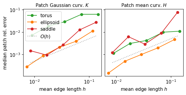

Region averages converge, at roughly the \(O(h)\) rate the measure theory predicts, for all three surfaces — in contrast to the flat pointwise estimates. Two torus converges more slowly than the others — its mesh is the least regular.

7. Region-averaged metric and second fundamental form

The same holds for the first and second fundamental forms. We test the patch area from the metric (\(\sum_{f\in P}\tfrac12\sqrt{\det g}\) vs \(\int_P dA\)) and the patch mean curvature from the shape operator \(S=g^{-1}b\) built with elastic.get_second_fundamental_form (an area-weighted per-face average \(\sum_f H_f\,A_f/\sum_f A_f\) vs \(\int_P H\,dA\)). Faces are assigned to sectors by their centroid.

findfont: Font family 'normal' not found.
findfont: Font family 'normal' not found.
findfont: Font family 'normal' not found.
findfont: Font family 'normal' not found.
findfont: Font family 'normal' not found.
findfont: Font family 'normal' not found.
findfont: Font family 'normal' not found.
findfont: Font family 'normal' not found.
findfont: Font family 'normal' not found.
findfont: Font family 'normal' not found.
findfont: Font family 'normal' not found.
findfont: Font family 'normal' not found.
findfont: Font family 'normal' not found.
findfont: Font family 'normal' not found.
findfont: Font family 'normal' not found.
findfont: Font family 'normal' not found.
findfont: Font family 'normal' not found.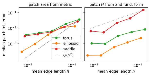

Both converge under region averaging: the metric area at \(O(h^2)\), and the second-fundamental- form mean curvature at \(\sim O(h)\) — even though the mid-edge-normal second fundamental form has an \(O(1)\) per-face noise floor pointwise. Averaging over a fixed region recovers a convergent quantity, consistent with the measure-convergence picture of §5.

Summary

quantity	operator	pointwise	region-averaged
gradient	`linops.compute_gradient_3d`	\(O(h)\) (exact on flat)	—
Laplace–Beltrami	`linops.compute_cotan_laplace`	\(O(h)\) (exact on flat)	—
Gaussian curvature \(K\)	`geom.get_gaussian_curvature`	stable, non-convergent	\(O(h)\)
mean curvature \(H\)	`geom.get_mean_curvature_laplace`	stable, non-convergent	\(O(h)\)
mean curvature (barycentric)	dihedral / barycentric area	worst pointwise	\(O(h)\) after averaging
metric / area	`elastic.get_metric`	area exact per triangle	patch area \(O(h^2)\)
2nd fundamental form	`elastic.get_second_fundamental_form`	\(O(1)\) per-face noise	patch \(H\) \(\sim O(h)\)

The differential operators (gradient, Laplace–Beltrami) converge pointwise. The curvature estimators do not converge pointwise on general meshes — but they are pointwise stable and converge in the measure / weak sense, i.e. integrated over fixed regions (Cohen-Steiner–Morvan 2003; Hildebrandt–Polthier–Wardetzky 2006). Delaunay-flipping the deformed meshes and normalising the error by the surface-mean magnitude \(\overline{|A|}\) are what make these trends clean and well-defined. No operator showed a bug: all match igl to machine precision.