rotation -

Find the 3D rotation that aligns data on the sphere. Part of pipeline for multiple recordings.

Here, we build tools to rotationally align data defined on a 2d-sphere using spherical harmonics. We consider the following problem: given two scalar functions \(f,h: S^2 \rightarrow \mathbb{R}\) on the sphere, find the rotation \(g\in O(3)\) that best aligns them, in the sense that it maximizes \(\int d\Omega f(x) h(g^{-1}x)\). We call \(f\) the source and \(h\) the target signal.

We expand the functions in terms of spherical harmonics, use the Wigner D-matrices to compute the effect of rotation, and find the best possible rotation via optimization.

In principle, the above could be done more efficiently using the fast spherical harmonics transform and the fast inverse Wigner transform. To minimize dependencies and keep the code simple, we won’t do that here, .

Spherical harmonics

We will represent spherical harmonics coefficients as dicts, indexed by total angular momentum \(l\), with an entry being a vector for the different \(m=-l,..., l\). Since we have real signals, we can get negative \(m\) from the positive ones.

---

spherical_to_cartesian

def spherical_to_cartesian(
    r, theta, phi
): # array of x/y/z coordinates. Last axis indexes coordinate axes.

Convert spherical coordinates to cartesian coordinates.

Uses en.wikipedia.org/wiki/Spherical_coordinate_system convention.

---

cartesian_to_spherical

def cartesian_to_spherical(
    arr, # array of x/y/z coordinates. last axis indexes coordinate axes.
): # r, theta, phi spherical coordinates

Convert cartesian coordinates to spherical coordinates.

Uses en.wikipedia.org/wiki/Spherical_coordinate_system convention.

# let's get a test case - a mesh obtained by mapping a mesh conformally to the sphere

mesh = tcmesh.ObjMesh.read_obj("datasets/movie_example/map_to_sphere.obj")
mesh_3d = tcmesh.ObjMesh.read_obj("datasets/movie_example/final_uv.obj")

# as test signal, let's use the log(areas) of the mesh triangles

areas_sphere = igl.doublearea(mesh.vertices, mesh.tris)
areas_3d = igl.doublearea(mesh_3d.vertices, mesh_3d.tris)

signal = np.log(areas_sphere/areas_3d)
signal -= signal.mean()

centroids = mesh.vertices[mesh.tris].mean(axis=1)
r, theta, phi = cartesian_to_spherical(centroids)

plt.scatter(phi, theta, c=signal, s=1, vmin=-3, vmax=3)
plt.axis("equal");

np.allclose(spherical_to_cartesian(r, theta, phi), centroids)

True

## Interpolate onto a grid as a check

n_grid = 256
phi_grid, theta_grid = np.meshgrid(np.linspace(-np.pi,np.pi, 2*n_grid), np.linspace(0, np.pi, n_grid)[::-1], )
interpolated = interpolate.griddata(np.stack([phi, theta], axis=-1), signal,
                                    (phi_grid, theta_grid), method='linear')
dTheta = np.pi/(n_grid-1)
dPhi = 2*np.pi/(2*n_grid-1)
interpolated = np.nan_to_num(interpolated)

plt.imshow(interpolated, vmin=-2.75, vmax=2.75)

# Check normalization and orthogonality of spherical harmonics for grid

print(np.sum(np.abs(special.sph_harm(1, 2, phi_grid, theta_grid))**2 * np.sin(theta_grid) * dTheta * dPhi))
print(np.abs(np.sum(special.sph_harm(2, 3, phi_grid, theta_grid)
              *np.conjugate(special.sph_harm(2, 4, phi_grid, theta_grid))
              *np.sin(theta_grid)*dTheta*dPhi)))

1.0019569486052557
1.0290434898119816e-16

# Check the relation between negative and positive m. Keep in mind (-1)^m factor

l, m = (4, 3)
np.allclose((-1)**(-m) * np.conjugate(special.sph_harm(m, l, phi_grid,theta_grid)),
            special.sph_harm(-m, l, phi_grid,theta_grid))

True

# Now let's do the direct calculation without extra interpolation. Check orthonormality

weights = igl.doublearea(mesh.vertices, mesh.tris)/2

print(np.sum(np.abs(special.sph_harm(1, 2, phi, theta))**2 * weights))
print(np.abs(np.sum(special.sph_harm(2, 3, phi, theta)
              *np.conjugate(special.sph_harm(2, 4, phi, theta))
              *weights)))

0.999525046106509
0.00010996886047295266

---

compute_spherical_harmonics_coeffs

def compute_spherical_harmonics_coeffs(
    f, # Sample values
    phi, # Sample point azimuthal coordinates
    theta, # Sample point longditudinal coordinates
    weights, # Sample weights. For instance, if you have a function sampled on a regular phi-theta grid,
this should be dTheta*dPhi*np.sin(theta)
    max_l, # Maximum angular momentum
): # Dictionary, indexed by total angular momentum l=0 ,..., max_l-1. Each entry is a vector
of coefficients for the different values of m=-2l,...,2*l

Compute spherical harmonic coefficients for a scalar real-valued function defined on the unit sphere.

Takes as input values of the function at sample points (and sample weights), and computes the overlap with each spherical harmonic by “naive” numerical integration.

Since the function is assumed real, we have f^{l}{-m} = np.conjugate(f^{l}{m}).

weights_grid = np.sin(theta_grid)*dTheta*dPhi
spherical_harmonics_coeffs = compute_spherical_harmonics_coeffs(interpolated, phi_grid, theta_grid,
                                                                weights_grid, max_l=15)

CPU times: user 1.81 s, sys: 3.1 ms, total: 1.82 s
Wall time: 1.81 s

spherical_harmonics_coeffs[3]

array([-0.24842273+0.41967878j,  0.32333336-0.37140101j,
        0.24521225-0.18171839j, -0.38792664-0.j        ,
       -0.24521225-0.18171839j,  0.32333336+0.37140101j,
        0.24842273+0.41967878j])

---

spherical_harmonics_to_grid

def spherical_harmonics_to_grid(
    coeffs, # Dictionary, indexed by total angular momentum l=0 ,..., max_l. Each entry is a vector
of coefficients for the different values of m=-2l,...,2*l
    n_grid:int=256
): # Reconstructed signal interpolated on rectangular phi-theta grid

Compute signal on rectangular phi-theta grid given spherical harmonics coefficients.

Assumes underlying function is real-valued

reconstructed = spherical_harmonics_to_grid(spherical_harmonics_coeffs, n_grid=256)

np.abs(reconstructed.imag).mean(), np.abs(reconstructed.real).mean() # as

(2.2578012798576635e-17, 1.7509102818359779)

plt.imshow(reconstructed.real, vmin=-2.75, vmax=2.75)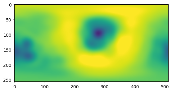

## now without the extra interpolation step

max_l = 15

weights = igl.doublearea(mesh.vertices, mesh.tris)/2
spherical_harmonics_coeffs_direct = compute_spherical_harmonics_coeffs(signal, phi, theta, weights,
                                                                       max_l=max_l)

reconstructed_direct = spherical_harmonics_to_grid(spherical_harmonics_coeffs_direct, n_grid=256)

plt.imshow(reconstructed_direct.real, vmin=-2.75, vmax=2.75)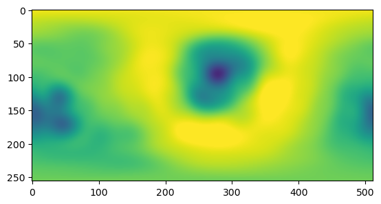

Rotational alignment

As a test, let’s randomly rotate our signal.

rot_mat = stats.special_ortho_group.rvs(3)
rot_mat

array([[ 0.01887775,  0.81035922, -0.5856292 ],
       [ 0.89941855,  0.24206006,  0.36394121],
       [ 0.43668055, -0.53359616, -0.72428256]])

mesh_rotated = deepcopy(mesh)
mesh_rotated.vertices = mesh_rotated.vertices @ rot_mat.T

areas_sphere_rotated  = igl.doublearea(mesh_rotated.vertices , mesh.tris)

signal_rotated = np.log(areas_sphere_rotated/areas_3d)
signal_rotated -= signal_rotated.mean()

centroids_rotated = mesh_rotated.vertices[mesh_rotated.tris].mean(axis=1)
_, theta_rotated, phi_rotated = cartesian_to_spherical(centroids_rotated)

plt.scatter(phi_rotated, theta_rotated, c=signal_rotated , s=1, vmin=-3, vmax=3)
plt.axis("equal");

weights_rotated = igl.doublearea(mesh_rotated.vertices, mesh.tris)/2
spherical_harmonics_coeffs_rotated = compute_spherical_harmonics_coeffs(signal_rotated,
                                                                        phi_rotated, theta_rotated,
                                                                        weights_rotated, max_l=max_l)

# let's check that the power per band is conserved
power_direct = {key: np.sum(np.abs(val)**2) for key, val in spherical_harmonics_coeffs_direct.items()}
power_rotated = {key: np.sum(np.abs(val)**2) for key, val in spherical_harmonics_coeffs_rotated.items()}

power_direct

{0: 31.75093316228961,
 1: 1.0569845383858716,
 2: 7.656637801049782,
 3: 1.2934800832192117,
 4: 1.1934413112502484,
 5: 0.16200066481681066,
 6: 0.050219817507973934,
 7: 0.03481762596812547,
 8: 0.01422448292437451,
 9: 0.04835575407817688,
 10: 0.01666320569699937,
 11: 0.04036958829270747,
 12: 0.0241966285740686,
 13: 0.024417478492580472,
 14: 0.015292984314499655}

power_rotated

{0: 31.75093316228961,
 1: 1.0569845383858694,
 2: 7.656637801049786,
 3: 1.29348008321921,
 4: 1.1934413112502456,
 5: 0.16200066481681097,
 6: 0.05021981750797396,
 7: 0.034817625968125335,
 8: 0.014224482924374391,
 9: 0.048355754078175966,
 10: 0.016663205696999295,
 11: 0.04036958829270838,
 12: 0.02419662857406937,
 13: 0.024417478492580014,
 14: 0.015292984314499138}

Inference of the rotation matrix from the spherical harmonics

Now for the difficult part. We need to infer the rotation matrix. The spherical harmonics will transform as blocks for each \(l\). Wigner D-matrices describe how. The code below is based on https://github.com/moble/spherical.

# Load the spherical module for comparison, even though we will re-implement it to minimize dependencies

import quaternionic
import spherical

# Indeed, using the correct Wigner matrix can undo our rotation

wigner = spherical.Wigner(15)
D = wigner.D(quaternionic.array.from_rotation_matrix(rot_mat))

l = 5
mp = 3

np.sum([D[wigner.Dindex(l, mp, m)]*spherical_harmonics_coeffs_direct[l][l+m]
        for m in range(-l, l+1)]), spherical_harmonics_coeffs_rotated[l][l+mp]

((0.0014361876877559377+0.11925102266293089j),
 (0.0014361876877558369+0.11925102266292989j))

Quaternions and rotation

Rotations can be respresensted by unit quaternion \(\mathbf{q}=(q_1, q_i, q_j, q_k)\). The spatial part \((q_i,q_j,q_k)\) defines the orientation of the rotation axis, and \(\alpha=2\arccos(u_1)\) is the rotation angle. For a unit vector \(\mathbf{u}\) defining the orientation of rotation and rotation angle \(\alpha\): \[q = \sin(\alpha/2) \mathbf{u} + \cos(\alpha/2)\] See https://fr.wikipedia.org/wiki/Quaternions_et_rotation_dans_l%27espace

---

quaternion_power

def quaternion_power(
    q, n
):

Raise quaternion to an integer power, potentially negative

---

multiply_quaternions

def multiply_quaternions(
    q, p
):

Call self as a function.

---

invert_quaternion

def invert_quaternion(
    q
):

Invert a quaternion

---

conjugate_quaternion

def conjugate_quaternion(
    q
):

Conjugate a quaternion

---

quaternion_to_complex_pair

def quaternion_to_complex_pair(
    q
):

Convert quaternion to pair of complex numbers q0+iq3, q2+iq1

---

rot_mat_to_quaternion

def rot_mat_to_quaternion(
    Q
):

Convert 3d rotation matrix into unit quaternion.

If determinant(Q) = -1, returns the unit quaternion corresponding to -Q

See https://fr.wikipedia.org/wiki/Quaternions_et_rotation_dans_l%27espace

---

quaternion_to_rot_max

def quaternion_to_rot_max(
    q
):

Convert unit quaternion into a 3d rotation matrix.

See https://fr.wikipedia.org/wiki/Quaternions_et_rotation_dans_l%27espace

Q = stats.special_ortho_group.rvs(3)
print(Q)

[[-0.1132397  -0.71935166 -0.6853539 ]
 [-0.98651227  0.16346272 -0.00857196]
 [ 0.11819607  0.67513934 -0.7281597 ]]

np.array(quaternionic.array.from_rotation_matrix(Q))/rot_mat_to_quaternion(Q)

array([-1., -1., -1., -1.])

q = rot_mat_to_quaternion(Q)
Q_back = quaternion_to_rot_max(q)
np.allclose(Q_back, Q)

True

Q1 = stats.special_ortho_group.rvs(3)
Q2 = stats.special_ortho_group.rvs(3)

R1 = quaternionic.array.from_rotation_matrix(Q1)
R2 = quaternionic.array.from_rotation_matrix(Q2)

R1 * R2

quaternionic.array([-0.55563224, -0.13607597,  0.55312392, -0.60564847])

multiply_quaternions(rot_mat_to_quaternion(Q1), rot_mat_to_quaternion(Q2))

array([-0.55563224, -0.13607597,  0.55312392, -0.60564847])

R1**4

quaternionic.array([ 0.97660873, -0.05627274, -0.19008602,  0.08328306])

q = rot_mat_to_quaternion(Q1)
quaternion_power(q, 4)

array([ 0.97660873, -0.05627274, -0.19008602,  0.08328306])

Wigner D-matrix as a function of quaternions

We use this formula: https://spherical.readthedocs.io/en/main/WignerDMatrices/:

image.png

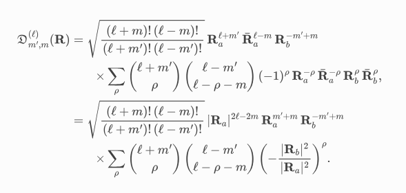
To execute it rapidly, it is best to pre-compute the combinatorial coefficients via a recursion.

---

get_binomial_matrix

def get_binomial_matrix(
    N_max
):

Get N_max by N_max matrix with entries binomial_matrix[i, j] = (i choose j).

Computed via Pascal’s triangle.

get_binomial_matrix(20)

46.9 μs ± 604 ns per loop (mean ± std. dev. of 7 runs, 10,000 loops each)

get_binomial_matrix(20)[12, 3], special.comb(12, 3)

(220.0, 220.0)

---

get_wigner_D_matrix

def get_wigner_D_matrix(
    q, l, binomial_matrix:NoneType=None
):

Get (2l+1, 2l+1) Wigner D matrix for angular momentum l and rotation (unit quatertion) q

mat = get_wigner_D_matrix(q, l=10) 
# 30 ms. all. down to 2 by binomial recursion

3.73 ms ± 32.9 μs per loop (mean ± std. dev. of 7 runs, 100 loops each)

get_wigner_D_matrix(q, l=10)[12, 2]

(0.3103085067597108-0.1994583649968599j)

Q = stats.special_ortho_group.rvs(3)
q = rot_mat_to_quaternion(Q)

# q = np.array([ 0.99950656,  0.        ,  0.        , -0.03141076]) # special case: important to check

# compare with the spherical package. looks pretty good, small diff if q[0]==0

wigner = spherical.Wigner(15)
#D = wigner.D(quaternionic.array.from_rotation_matrix(Q))
D = wigner.D(q)

l = 2
binomial_matrix = get_binomial_matrix(2*l)
mp, m = (0, 0)

(D[wigner.Dindex(l, mp, m)],
 _get_wigner_D_element(*quaternion_to_complex_pair(q), l, mp, m, binomial_matrix),)

((-0.2254678510932408+0j), (-0.22546785109324072+0j))

mat = get_wigner_D_matrix(q, l=10) 
# a little slow

CPU times: user 3.44 ms, sys: 85 μs, total: 3.53 ms
Wall time: 3.52 ms

---

overlap_spherical_harmonics

def overlap_spherical_harmonics(
    coeffsA, coeffsB, normalized:bool=False
):

Compute overlap (L2 inner product) between two sets of spherical harmonics.

Optionally, normalize by the norm of coeffsA, coeffsB.

---

rotate_spherical_harmonics_coeffs

def rotate_spherical_harmonics_coeffs(
    R, # Rotation matrix, may be improper. If you have a quaternion,
 use quaternion_to_rot_mat.
    coeffs, # Dictionary, indexed by total angular momentum l=0 ,..., max_l-1. Each entry is a vector
of coefficients for the different values of m=-2l,...,2*l
): # Rotated spherical harmonics coefficients.

Rotate spherical harmonics by the given (improper or proper) rotation matrix.

Uses Wigner-D matrices. Don’t use this function in an optimization context - you can in general save a bunch of time by reusing D-matrices etc.

---

parity_spherical_harmonics_coeffs

def parity_spherical_harmonics_coeffs(
    coeffs, # Dictionary, indexed by total angular momentum l=0 ,..., max_l-1. Each entry is a vector
of coefficients for the different values of m=-2l,...,2*l
): # Parity-transformed spherical harmonics coefficients.

Apply parity operator to spherical harmonics coefficients.

Parity means (x,y,z) -> (-x,-y,-z) and f^l_m -> (-1)^m * f^l_m.

# Check that the Wigner D correctly re-aligns our harmonic coefficients

l = 7
D_matrix = get_wigner_D_matrix(rot_mat_to_quaternion(rot_mat), l=l)

np.allclose(D_matrix@spherical_harmonics_coeffs_direct[l], spherical_harmonics_coeffs_rotated[l])
# success!

True

# before alignment, the coefficients are different
not np.allclose(spherical_harmonics_coeffs_direct[l], spherical_harmonics_coeffs_rotated[l])

True

Cross-correlation analysis

We now want to find the rotation that maximizes the cross-correlation between the two signals. To do so, we compute the overlap for several trial rotations to get an initial guess and refine it by optimization.

# This is how you compute the overlap, here using my code

max_l = 10
binomial_matrix = get_binomial_matrix(2*max_l)
R = np.copy(rot_mat)

corr_coeff = 0
for l in range(0, max_l):
    D_matrix = get_wigner_D_matrix(rot_mat_to_quaternion(R), l=l, binomial_matrix=binomial_matrix)
    corr_coeff += np.sum(D_matrix@spherical_harmonics_coeffs_direct[l]
                         *np.conjugate(spherical_harmonics_coeffs_rotated[l]))

CPU times: user 10.6 ms, sys: 18 μs, total: 10.6 ms
Wall time: 10.4 ms

corr_coeff

(43.26109524149018+2.5746956649943757e-16j)

Now let’s consider multiple rotations. we can save time by minimizing the number of times we compute the D-matrix by using the fact that \(D(R^n) = D(R)^n\) - hence, for every rotation axis, we can try out a large number of rotation angles efficiently.

D_mat = get_wigner_D_matrix(rot_mat_to_quaternion(R), l=2)
D_mat_of_square = get_wigner_D_matrix(rot_mat_to_quaternion(R@R), l=2)
np.allclose(D_mat@D_mat, D_mat_of_square)

True

Sampling the sphere

How do we get a good sampling of unit vectors on the sphere as rotation axes for our initial guess? Let’s use an “icosphere” https://en.wikipedia.org/wiki/Geodesic_polyhedron

---

get_icosphere

def get_icosphere(
    subdivide:int=0
):

Return the icosphere triangle mesh with 42 regularly spaced vertices on the unit sphere.

Optionally, subdivide mesh n times, increasing vertex count by factor 4^n.

---

rotation_alignment_brute_force

def rotation_alignment_brute_force(
    sph_harmonics_source, # Dictionary, indexed by total angular momentum l=0 ,..., max_l. Each entry is a vector
of coefficients for the different values of m=-2l,...,2*l. Source signal, to be
transformed.
    sph_harmonics_target, # Dictionary, indexed by total angular momentum l=0 ,..., max_l. Each entry is a vector
of coefficients for the different values of m=-2l,...,2*l. Target signal.
    max_l:NoneType=None, # Maximum angular momentum. If None, the maximum value available in the input
spherical harmonics is used.
    n_angle:int=100, # Number of trial rotation angles [0,..., 2*pi]
    n_subdiv_axes:int=1, # Controls the number of trial rotation axes. Rotation axes are vertices of
the icosphere which can be subdivided. There will be roughly
40*4**n_subdiv_axes trial axes. This parameter has the strongest influence
on the run time.
    allow_flip:bool=False, # Whether to allow improper rotations with determinant -1. In this case, 
we return _two_ sets of overlaps and rotation matrices, one for the best
proper, and one for the best improper rotation.
): # optimal_trial_rotation : (3,3) np.array
    Best trial rotation as rotation matrix.
overlap : float
    Normalized overlap. 1=perfect alignment.

Compute rotational alignment between two signals on the sphere by brute force.

The two signals have to be represented by their spherical harmonics coefficients. Uses Wigner-D matrices to calculate the overlap between the two signals for a set of rotations and finds the rotation that maximizes the overlap.

The trial rotations are generated by taking a set of approx. equidistant points on the 2d sphere as rotation axes, and a set of equally spaced angles [0,…, 2*pi] as rotation angles.

The rotation is such that it transforms the source signal to match the target.

# let's set up our example

#rot_mat = -np.eye(3)
#rot_mat = stats.special_ortho_group.rvs(3)
rot_mat = -stats.special_ortho_group.rvs(3)

rot_mat, np.linalg.det(rot_mat)

(array([[ 0.93858452, -0.25998611, -0.22686191],
        [ 0.29335272,  0.94740493,  0.12793776],
        [-0.18166805,  0.18663096, -0.96548724]]),
 -1.0000000000000004)

mesh_rotated = deepcopy(mesh)
mesh_rotated.vertices = mesh_rotated.vertices @ rot_mat.T
signal_rotated = np.copy(signal)

centroids_rotated = mesh_rotated.vertices[mesh_rotated.tris].mean(axis=1)
_, theta_rotated, phi_rotated = cartesian_to_spherical(centroids_rotated)

weights_rotated = igl.doublearea(mesh_rotated.vertices, mesh.tris)/2
spherical_harmonics_coeffs_rotated = compute_spherical_harmonics_coeffs(signal_rotated,
                                                                        phi_rotated, theta_rotated,
                                                                        weights_rotated, max_l=max_l)

R_opt, overlap, R_opt_flipped, overlap_flipped = rotation_alignment_brute_force(spherical_harmonics_coeffs_direct,
                                                                                 spherical_harmonics_coeffs_rotated,
                                                            max_l=10, n_angle=100, n_subdiv_axes=2, allow_flip=True)

rot_mat_to_quaternion(R_opt_flipped), rot_mat_to_quaternion(rot_mat), overlap, overlap_flipped

CPU times: user 3.62 s, sys: 0 ns, total: 3.62 s
Wall time: 3.62 s

(array([ 0.15643447, -0.07492257,  0.13505986, -0.97553765]),
 array([ 0.14097676, -0.10408312,  0.08014416, -0.98125897]),
 (0.9910003623902994+7.84107514069421e-17j),
 (0.9931975537491813+6.548624948738893e-17j))

np.linalg.norm(R_opt-rot_mat), np.linalg.norm(R_opt_flipped-rot_mat)

(2.0000958259305763, 0.18184532747844342)

---

rotation_alignment_refined

def rotation_alignment_refined(
    sph_harmonics_source, # Dictionary, indexed by total angular momentum l=0 ,..., max_l. Each entry is a vector
of coefficients for the different values of m=-2l,...,2*l. Source signal, to be
transformed.
    sph_harmonics_target, # Dictionary, indexed by total angular momentum l=0 ,..., max_l. Each entry is a vector
of coefficients for the different values of m=-2l,...,2*l. Target signal.
    R_initial, # Initial rotation as a rotation matrix
    max_l:NoneType=None, # Maximum angular momentum. If None, the maximum value available in the input
spherical harmonics is used.
    maxfev:int=100, # Number of function evaluations during optimization. This parameter has
the strongest influence on the run time.
): # optimal_rotation : (3, 3) np.array
    Best rotation as rotation matrix. Will always have the same determinant (i.e. -1, 1)
    as the initial guess.
overlap : float
    Normalized overlap. 1=perfect alignment.

Refine rotational alignment between two signals on the sphere by optimization.

The two signals have to be represented by their spherical harmonics coefficients. Uses Wigner-D matrices to calculate the overlap between the two signals and uses Nelder-Mead optimization to find the best one.

Requires a good initial guess for the rotation, as created by rotation_alignment_brute_force.

The rotation is such that it transforms the source signal to match the target.

R_refined, overlap_refined = rotation_alignment_refined(spherical_harmonics_coeffs_direct,
                                                        spherical_harmonics_coeffs_rotated, R_opt_flipped,
                                                        max_l=10, maxfev=200)

rot_mat_to_quaternion(R_refined), np.linalg.det(R_refined), overlap_refined

CPU times: user 1.74 s, sys: 20 ms, total: 1.76 s
Wall time: 1.75 s

(array([ 0.14097678, -0.10408313,  0.08014421, -0.98125896]),
 -0.9999999999999999,
 0.9999999999999993)

np.linalg.norm(R_refined-rot_mat)

1.5330429766260706e-07

---

rotational_alignment

def rotational_alignment(
    sph_harmonics_source, # Dictionary, indexed by total angular momentum l=0 ,..., max_l. Each entry is a vector
of coefficients for the different values of m=-2l,...,2*l. Source signal, to be
transformed.
    sph_harmonics_target, # Dictionary, indexed by total angular momentum l=0 ,..., max_l. Each entry is a vector
of coefficients for the different values of m=-2l,...,2*l. Target signal.
    allow_flip:bool=False, # Whether to allow improper rotations with determinant -1. 
    max_l:NoneType=None, # Maximum angular momentum. If None, the maximum value available in the input
spherical harmonics is used.
    n_angle:int=100, # Number of trial rotation angles [0,..., 2*pi]
    n_subdiv_axes:int=1, # Controls the number of trial rotation axes. Rotation axes are vertices of
the icosphere which can be subdivided. There will be roughly
40*4**n_subdiv_axes trial axes. This parameter has the strongest influence
on the run time.
    maxfev:int=100, # Number of function evaluations during fine optimization.
): # optimal_rotation : (3, 3) np.array
    Best rotation as rotation matrix. Will always have the same determinant (i.e. -1, 1)
    as the initial guess.
overlap : float
    Normalized overlap. 1=perfect alignment.

Rotational alignment between two signals on the sphere.

The two signals have to be represented by their spherical harmonics coefficients. Uses Wigner-D matrices to calculate the overlap between the two signals.

Alignment happens in two steps: first, a coarse alignment using a large number of trial rotation axes and angles, and then refinement via optimization.

The rotation is such that it transforms the source signal to match the target.

R_refined, overlap = rotational_alignment(spherical_harmonics_coeffs_direct, spherical_harmonics_coeffs_rotated,
                                          max_l=10, n_angle=100, n_subdiv_axes=1, maxfev=200,
                                          allow_flip=True)

np.linalg.norm(R_refined-rot_mat), np.round(np.linalg.det(R_refined)), overlap

CPU times: user 4.49 s, sys: 35 μs, total: 4.49 s
Wall time: 4.48 s

(1.5571961945381298e-07, -1.0, 0.999999999999998)

How well does this work?

Looks pretty good! I find that using about 160 trial rotation axes in the brute force step (subdiv=1) is a good choice - fewer trial axes lead to poor initial guesses.

However, the first guess can often get the parity wrong! Therefore, it is best to run brute force and fine alignment for both parities, and then choose which one is better.