Morph one surface mesh onto another via map to reference shape (disk, sphere). Part of the pipeline for dynamic data.
In this notebook, we present some additional wrapping algorithms. So far, we have wrapped two meshes by simply projection each source mesh vertex onto the closest position on the target mesh and carrying out some on-surface smoothing. This works but is not necessarily extremely robust, and can lead to very deformed UV maps when there are large, localized deformations.
Here, we’ll implement an alternative algorithm that works by (a) mapping each mesh into a common reference in a mathematically standardized way -harmonic maps- and then (b) chaining together the map from the source mesh to the common reference and from the reference to the target mesh to get a surface-surface map.
We provide algorithms for meshes of disk, cylindrical, and spherical topology (potentially with holes). For arbitrary genus (i.e. handles, like a torus), one can take a look at hyperbolic orbifolds https://github.com/noamaig/hyperbolic_orbifolds/. Not implemented here.
Loading test data
Let’s load the test meshes from the fly midgut dataset.
mesh_initial_UV = tcmesh.ObjMesh.read_obj("datasets/movie_example/initial_uv.obj")mesh_final_UV = tcmesh.ObjMesh.read_obj("datasets/movie_example/final_uv.obj") # this is a UV map defined for tpt 20mesh_1 = tcmesh.read_other_formats_without_uv(f"datasets/movie_example/meshes/mesh_{str(1).zfill(2)}.ply")mesh_2 = tcmesh.read_other_formats_without_uv(f"datasets/movie_example/meshes/mesh_{str(2).zfill(2)}.ply")mesh_60 = tcmesh.read_other_formats_without_uv(f"datasets/movie_example/meshes/mesh_{str(60).zfill(2)}.ply")
Warning: readOBJ() ignored non-comment line 4:
  o mesh_01_cylinder_seams_uv
Warning: readOBJ() ignored non-comment line 3:
  o mesh_20_uv
Disk
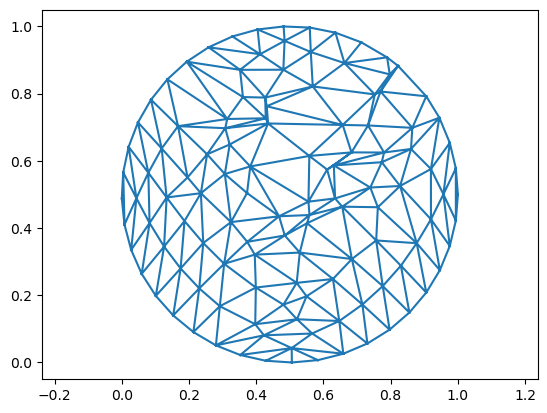
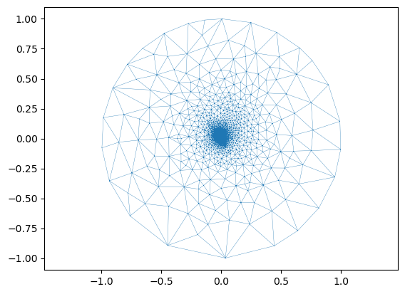
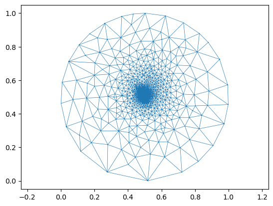
Following https://libigl.github.io/libigl-python-bindings/tut-chapter4/. We first map each mesh to the unit disk using harmonic coordinates. Boundary conditions are such that the boundary loop is mapped to the unit circle isometrically (i.e. relative distances are preserved).
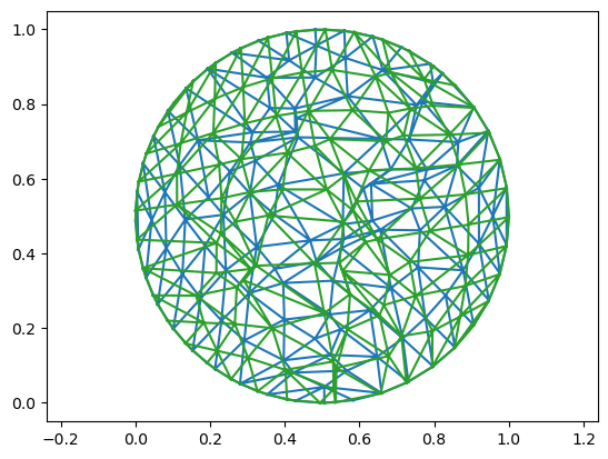
There is still a remaining rotation degree of freedom. This is fixed by optimizing the match of the conformal factors (i.e. the area distortion of the maps to the disk) using phase correlation.
map_to_disk
def map_to_disk( mesh, # Mesh. Must be topologically a disk (potentially with holes),and should be triangular. bnd:NoneType=None, # Boundary to map to the unit circle. If None, computed automatically. set_uvs:bool=False, # whether to set the disk coordinates as UV coordinates of the mesh.): # 2d vertex coordinates mapping the mesh to the unit disk in [0,1]^1
Map mesh to unit disk by computing harmonic UV coordinates.
The longest boundary loop of the mesh is mapped to the unit circle. Follows https://libigl.github.io/libigl-python-bindings/tut-chapter4/. Note: the disk is centered at (1/2, 1/2).
“We next seek the rotation that best aligns the two parameterizations. To do so, we first sample the conformal factors of each mesh onto a regular spherical grid (Figure 6, top right). We then find the rotation that maximizes the correlation between conformal factors, via a fast spectral transform.”
get_rot_mat2d
def get_rot_mat2d( phi):
Get 2d rotation matrix with angle phi.
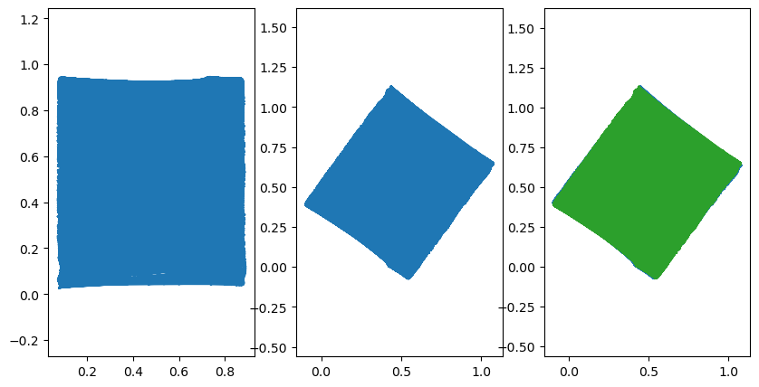
mesh_a = deepcopy(mesh)mesh_b = deepcopy(mesh)phi =-0.8*np.pimesh_b.texture_vertices = ((mesh_a.texture_vertices-np.array([0.5, 0.5]))@get_rot_mat2d(phi)+np.array([0.5, 0.5]))# test orientation flipflip = np.diag([-1,1])mesh_b.texture_vertices = ((mesh_b.texture_vertices-np.array([0.5, 0.5]))@flip+np.array([0.5, 0.5]))mesh_b.faces = [fc[::-1] for fc in mesh_b.faces]
def rotational_align_disk( mesh_source, # Mesh. Must be topologically a disk (potentially with holes),and should be triangular. mesh_target, # Mesh. Must be topologically a disk (potentially with holes),and should be triangular. disk_uv_source:NoneType=None, # Disk coordinates for each vertex in the source mesh. Optional.If None, the UV coordinates of mesh_source are used. disk_uv_target:NoneType=None, # Disk coordinates for each vertex in the target mesh. Optional.If None, the UV coordinates of disk_uv_target are used. allow_flip:bool=True, # Whether to allow flips (improper rotations). If a flipoccurs, np.linalg.det(rot_mat) <0 q:float=0.01, # Conformal factors are clipped at this quantile to avoid outliers. n_grid:int=1024, # Grid for interpolation of conformal factor during alignment): # new_texture_vertices_mesh_source : np.array Rotationally aligned texture verticesrot_mat : np.array of shape (2,2) Rotation matrixoverlap : float Overlap between aligned conformal factors. 1= perfect alignment.
Rotationally align two UV maps to the disk by the conformal factor.
Computes aligned UV coordinates. Assumes that the UV coordinates are in [0,1]^2. This works by computing the conformal factor (how much triangle size changes as it is mapped to the plane, and finding the optimal rotation to align the conformal factors via phase correlation.
mesh_a = deepcopy(mesh)mesh_b = deepcopy(mesh)phi =-0.8*np.pimesh_b.texture_vertices = ((mesh_a.texture_vertices-np.array([0.5, 0.5]))@get_rot_mat2d(phi)+np.array([0.5, 0.5]))flip = np.diag([-1,1])mesh_b.texture_vertices = ((mesh_b.texture_vertices-np.array([0.5, 0.5]))@flip+np.array([0.5, 0.5]))mesh_b.faces = [fc[::-1] for fc in mesh_b.faces]
def wrap_coords_via_disk( mesh_source, # Mesh. Must be topologically a disk (potentially with holes),and should be triangular. mesh_target, # Mesh. Must be topologically a disk (potentially with holes),and should be triangular. disk_uv_source:NoneType=None, # Disk coordinates for each vertex in the source mesh. Optional.If None, computed via map_to_disk. disk_uv_target:NoneType=None, # Disk coordinates for each vertex in target mesh. Optional.If None, computed via map_to_disk. align:bool=True, # Whether to rotationally align the parametrizations. If False, they are used as-is. q:float=0.01, # Conformal factors are clipped at this quantile to avoid outliers. n_grid:int=1024, # Grid for interpolation of conformal factor during alignment.Higher values increase alignment precision.): # New 3d vertex coordinates for mesh_source, lying on the surfacedefined by mesh_target
Map 3d coordinates of source mesh to target mesh via a disk parametrization.
Disk parametrization can be provided or computed on the fly via harmonic coordinates. If desired, the two disks are also rotationally aligned.
Map a cylinder to the disk: fill one boundary with an extra vertex, map to the disk harmonically, use Moebius to move the extra vertex to the disk center.
moebius_disk
def moebius_disk( pts, b):
Compute a Moebius transformation of the disk. Moves disk origin by b. pts.shape is (…, 2)
complex_to_xy
def complex_to_xy( arr):
Map x+iy to (x, y). Return shape==(…,2 )
xy_to_complex
def xy_to_complex( arr):
Map (x,y) to x+iy. arr.shape==(…,2 )
polygon_centroid
def polygon_centroid( pts):
See https://en.wikipedia.org/wiki/Centroid. pts.shape is (…, 2)
polygon_area
def polygon_area( pts):
Polygon area via shoe-lace formula. Assuming no self-intersection. pts.shape is (…, 2)
# map to disk via harmonic mapbnd_uv =1* igl.map_vertices_to_circle(filled_vertices, first_boundary)uv = igl.harmonic(filled_vertices, filled_tris, first_boundary, bnd_uv, 1)# map the center of the second boundary to disk centeruv = moebius_disk(uv, -uv[-1])
uv[-1] # last point -at the center of filled cylinder opening- is mapped to center of
def map_cylinder_to_disk( mesh, # Mesh. Must be topologically a disk (potentially with holes),and should be triangular. outer_boundary:str='longest', # Boundary to map to the unit circle. If "longest"/"shortest", the longer/shorter one is mapped to the unit circle. If int,the boundary containing the vertex defined by the intis used. first_boundary:NoneType=None, # First boundary loop of cylinder. If None, computed automatically. second_boundary:NoneType=None, # Second boundary loop of cylinder. If None, computed automatically. set_uvs:bool=False, # whether to set the disk coordinates as UV coordinates of the mesh. return_filled:bool=False, # Whether to return vertices and faces with filled hole.): # uv : np.array2d vertex coordinates mapping the mesh to the unit disk in [0,1]^1. If filled_vertices isTrue, the last entry is the coordinate of the added point.filled_vertices : np.array3d vertices with extra vertex to fill second boundaryfilled_faces : np.array Faces with added faces to fill the second boundary.
Map cylinder mesh to unit disk by computing harmonic UV coordinates.
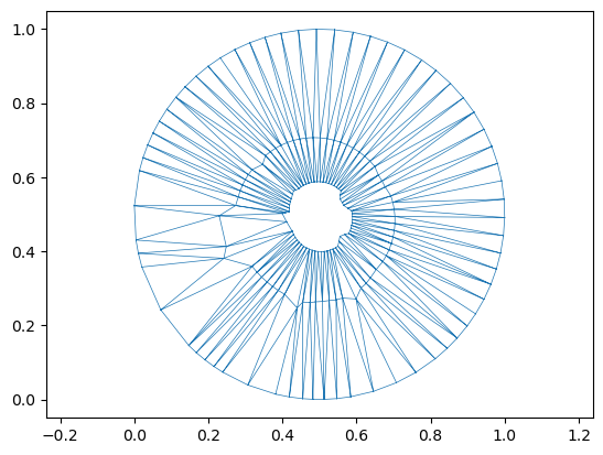
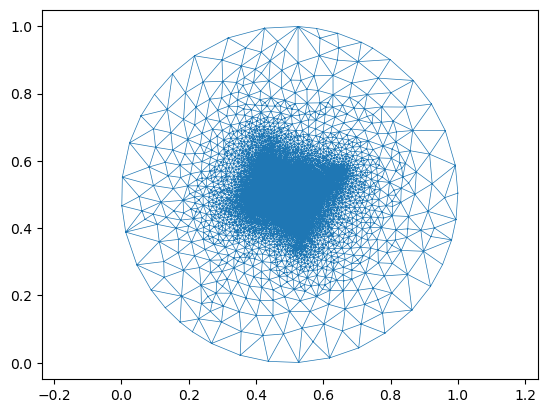
One boundary loop of the mesh is mapped to the circle with a diameter 1/2. The second boundary is filled by adding an extra vertex at its center, which is mapped to the disk center.
Which of the two circular boundaries is mapped to the center resp. the outer circle is set by the option outer_boundary.
## let's try a more challenging example - midgut mesh with two cuts to make it a cylindermesh = tcmesh.ObjMesh.read_obj("datasets/movie_example/mesh_1_cylinder_cut.obj") # cylinder_clean
Warning: readOBJ() ignored non-comment line 3:
  o mesh_01
def wrap_coords_via_disk_cylinder( mesh_source, # Mesh. Must be topologically a cylinder and should be triangular. mesh_target, # Mesh. Must be topologically a cylinder and should be triangular. q:float=0.01, # Conformal factors are clipped at this quantile to avoid outliers. n_grid:int=1024, # Grid for interpolation of conformal factor during alignment.Higher values increase alignment precision.): # new_coords : np.array New 3d vertex coordinates for mesh_source, lying on the surface defined by mesh_targetoverlap : float Measure of geometry overlap. 1= perfect alignment
Map 3d coordinates of source mesh to target mesh via an annulus parametrization.
Annulus parametrization can be provided or computed on the fly via harmonic coordinates. If desired, the two disks are also rotationally aligned. Meshes must be cylindrical. Two choices exist for mapping a cylinder to the plane (depending on which boundary circle is mapped to the disk boundary resp. center). Both options are tried, and the one leading to better alignment is used.
If you already have a map to the disk, use wrap_coords_via_disk instead.
For the sphere, we follow https://www.cs.cmu.edu/~kmcrane/Projects/MobiusRegistration/paper.pdf. The Riemann mapping theorem guarantees there is a conformal map of our surface to the unit sphere. This map is unique up to Moebius transformations (inversion about a point in the unit ball, and rotations). We fix the inversions by choosing the conformal map with the least amount of area distortion, and the rotation by registering the conformal factors as functions on the unit sphere using spherical harmonics
Cut sphere to disk by removing a single vertex
Map disk to plane conformally using harmonic coordinates. Turns out the least-squares conformal map is lousy at preserving angles (at least in igl)
Map disk to a sphere using stereographic projection, adding the removed vertex at the north pole
Fix Moebius inversion by choosing a conformal map with minimal distortion using Algorithm 1 from https://www.cs.cmu.edu/~kmcrane/Projects/MobiusRegistration/paper.pdf
Rotational registration using spherical harmonics (see notebook 03c)
Interpolation of vertex positions using spherical parametrization
mesh = deepcopy(mesh_final_UV)
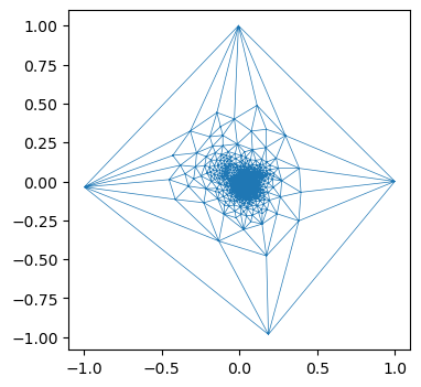
# this is what the map of the mesh sans north pole to the plane looks likefig = plt.figure(figsize=(4,4))plt.triplot(*uv.T, faces_disk, lw=0.5)
Strereographic projection
stereographic_sphere_to_plane
def stereographic_sphere_to_plane( pts):
Stereographic projection from unit sphere to plane from the north pole (0,0,1).
See https://en.wikipedia.org/wiki/Stereographic_projection. Convention: the plane is at z=0, unit sphere centered at the origin. pts should be an array of shape (…, 3)
stereographic_plane_to_sphere
def stereographic_plane_to_sphere( uv):
Stereographic projection from plane to the unit sphere from the north pole (0,0,1).
See https://en.wikipedia.org/wiki/Stereographic_projection. Convention: plane is at z=0, unit sphere centered at origin. uv should be an array of shape (…, 2)
Algorithm 1 from https://www.cs.cmu.edu/~kmcrane/Projects/MobiusRegistration/paper.pdf
center_moebius
def center_moebius( vertices_3d, # 3d mesh vertices vertices_sphere, # Initial vertex positions on unit sphere tris, # Faces of a triangular mesh n_iter_centering:int=10, # Centering algorithm iterations. alpha:float=0.5, # Learning rate. Lower values make the algorithm more stable): # vertices_sphere_centered : np.array of shape (n_verts, 3) Centered sphere coordinatescom_norm : float Distance of sphere vertex center of mass from origin. Low values indicate convergence of the algorithm.
Apply Moeboius inversions to minimize area distortion of a map from mesh to sphere.
Implementation of Algorithm 1 from: https://www.cs.cmu.edu/~kmcrane/Projects/MobiusRegistration/paper.pdf
Putting it all together …
map_to_sphere
def map_to_sphere( mesh, # Mesh. Must be topologically a sphere, and should be triangular. method:str='harmonic', # Method for computing the map from mesh without the north pole to the plane.Recommended: harmonic. R_max:int=100, # Maximum radius to consider when computing inverse stereographicprojection. If you get weird results, try a lower value. n_iter_centering:int=20, # Centering algorithm iterations. If 0, no centering is performed alpha:float=0.5, # Learning rate. Lower values make the centering algorithm more stable set_uvs:bool=False):
Compute a map of mesh to the unit sphere.
First, remove one vertex (the last one), and map the resulting disk-topology mesh to the plane using least squares conformal maps. Then map the plane to the sphere using stereographic projection.
The conformal map is chosen so that area distortion is as small as possible by (a) optimizing over the scale (“radius”) of the map to the disk and (b) “centering” the map using Algorithm 1 from cs.cmu.edu/~kmcrane/Projects/MobiusRegistration/paper.pdf.
This means the map is canonical up to rotations of the sphere.
angles_3d = igl.internal_angles(mesh.vertices, mesh.tris)angles_sphere = igl.internal_angles(coords_sphere, mesh.tris)np.nanmean(np.abs(angles_sphere.flatten()-angles_3d.flatten())) # map to sphere is close to conformal/angle-preserving
0.061201972212849245
Rotation alignment using rotation module
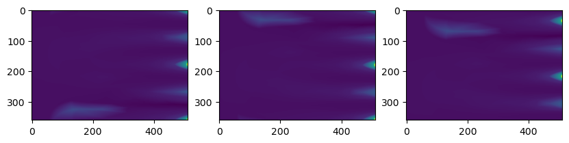
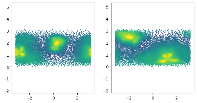
For a map to the sphere, we can compute the amount of area distortion at each point on the sphere. We can then use this “conformal factor” as a signal to rotationally align two maps (from different meshes) to the sphere.
# this is what the conformal factor (area distortion) looks like plotted vs phi, theta, for an example# (the same mesh mapped to the sphere, but arbitrarily rotated)fig, (ax1, ax2) = plt.subplots(ncols=2, figsize=(8, 4))ax1.scatter(phi_source, theta_source, c=signal_source, s=1, vmin=-3, vmax=3)ax2.scatter(phi_target, theta_target, c=signal_target, s=1, vmin=-3, vmax=3)ax1.axis("equal");ax2.axis("equal");
rotational_align_sphere
def rotational_align_sphere( mesh_source, # Mesh. Must be topologically a sphere (potentially with holes),and should be triangular. mesh_target, # Mesh. Must be topologically a sphere (potentially with holes),and should be triangular. coords_sphere_source, # Sphere coordinates for each vertex in the source mesh.If None, the UV coordinates are interpreted as angles 2*pi*u=phi,2*pi*v=theta. coords_sphere_target, # Sphere coordinates for each vertex in the source mesh.If None, the UV coordinates are interpreted as angles 2*pi*u=phi,2*pi*v=theta. allow_flip:bool=False, # Whether to allow improper rotations with determinant -1. max_l:int=10, # Maximum angular momentum. If None, the maximum value available in the inputspherical harmonics is used. n_angle:int=100, # Number of trial rotation angles [0,..., 2*pi] n_subdiv_axes:int=1, # Controls the number of trial rotation axes. Rotation axes are vertices ofthe icosphere which can be subdivided. There will be roughly40*4**n_subdiv_axes trial axes. This parameter has the strongest influenceon the run time. maxfev:int=100, # Number of function evaluations during fine optimization.): # coords_sphere_source_rotated : np.array Rotationally aligned sphere verticesrot_mat : np.array of shape (3,3) Rotation matrixoverlap : float How well the conformal factors overlap. 1= perfect overlap.
Rotationally align two UV maps to the sphere by the conformal factor.
Computes aligned spherical coordinates. Rotational alignment works by computing the conformal factor (how much triangle size changes as it is mapped to the sphere) and optimizing over rotations to find the one which leads to the best alignment. This works via an expansion in spherical harmonics. See tcrot.rotational_alignment
# first test case: same mesh, but map to the sphere rotatatedmesh_source = deepcopy(mesh_final_UV)mesh_target = deepcopy(mesh_final_UV)coords_sphere_source = map_to_sphere(mesh_source)rot_mat = stats.special_ortho_group.rvs(3)coords_sphere_target = coords_sphere_source @ rot_mat.T
# second test case: meshes for two frames of a moviemesh_source = deepcopy(mesh_2) # mesh_final_UVmesh_target = deepcopy(mesh_1) # mesh_initial_UVcoords_sphere_source = map_to_sphere(mesh_source)coords_sphere_target = map_to_sphere(mesh_target)
Now that we have (a) mapped both meshes to the sphere, (b) minized distortion via Moebius centering, and (c) rotationally aligned the two maps via spherical harmonics, we can interpolate the coordinates of mesh B onto mesh A.
wrap_coords_via_sphere
def wrap_coords_via_sphere( mesh_source, # Mesh. Must be topologically a disk (potentially with holes),and should be triangular. mesh_target, # Mesh. Must be topologically a disk (potentially with holes),and should be triangular. coords_sphere_source:NoneType=None, # Sphere coordinates for each vertex in the source mesh. Optional.If None, computed via map_to_sphere. coords_sphere_target:NoneType=None, # Sphere coordinates for each vertex in the target mesh. Optional.If None, computed via map_to_sphere. method:str='harmonic', # Method for comuting the map from sphere without north pole to plane n_iter_centering:int=10, # Centering algorithm iterations for computing map to the sphere. If 0, no centering is performed alpha:float=0.5, # Learning rate for computing map to the sphere. Lower values make the centering algorithm more stable. align:bool=True, # Whether to rotationally align the parametrizations. If False, they are used as-is. allow_flip:bool=False, # Whether to allow improper rotations with determinant -1 for rotational alignment. max_l:int=10, # Maximum angular momentum. If None, the maximum value available in the inputspherical harmonics is used. n_angle:int=100, # Number of trial rotation angles [0,..., 2*pi] n_subdiv_axes:int=1, # Controls the number of trial rotation axes. Rotation axes are vertices ofthe icosphere which can be subdivided. There will be roughly40*4**n_subdiv_axes trial axes. This parameter has the strongest influenceon the run time. maxfev:int=100, # Number of function evaluations during fine optimization for rotational alignment.): # new_coords : np.array New 3d vertex coordinates for mesh_source, lying on the surface defined by mesh_targetoverlap : np.array Overlap of conformal factor (area distortion) on sphere of the two meshes. Only returned if align isTrue.1 indicates perfect overlap.
Map 3d coordinates of source mesh to target mesh via a sphere parametrization.
Sphere parametrizations can be provided or computed on the fly using the least-area distorting conformal map to the sphere (see map_to_sphere). If desired, the two parametrizations are also aligned with respect to 3d rotations using mesh shape, using spherical harmonics. See rotational_align_sphere for details.
Try it out first using trimesh, then do myself to avoid dependency. Use trimesh.registration.nricp_sumner
-> No good, takes forever and my laptop runs out of memory. Also lots of parameters to tune whose meaning I don’t know.
Laplace Beltrami descriptors
Idea - compute the eigenfunctions \(\phi_i\) of the Laplace operator \(\Delta\) on the surface, and the embed each point \(p\) on the surface as \(p\mapsto \phi_i(p)/\sqrt{\lambda_i}\).
Not suitable - the spectral shapes of the midgut example mesh become extremely degenerate.
See https://www.cs.jhu.edu/~misha/ReadingSeminar/Papers/Rustamov07.pdf, https://web.archive.org/web/20100626223753id_/http://www.cs.jhu.edu/~misha/Fall07/Notes/Rustamov07.pdf
Functional mapping
[https://people.csail.mit.edu/jsolomon/assets/fmaps.pdf] - uses Laplace Beltrami descriptors. There appears to be an existing implementation in python. Let’s try out their example notebook
It does not work that well. Ok for matching from mapping timepoints 1->2, bad for 1->20, or 20->30. I get “patchy correspondences”: the map mesh A -> mesh B is not continuous and tears up mesh A into multiple patches that are stitched together in somewhat random order on mesh B. Also kinda slow.
As Dillon pointed out, shape descriptors of Laplace-Beltrami kind fundamentally use metric information. Laplace Beltrami is equivalent to a metric. Good for isometric deformations, like joint movements, bad for non-isometric, which is often the case for us.
So in principle, this is a nice method, but not quite what we need.