10. 3D Image analysis with cartographic projections
Note: this tutorial is currently a stub - sorry!
A main advantage of cartographically projecting 3D data to 2D is that it makes quantitative analysis significantly easier, for example:
- segmenting cells and measuring their shape
- quantifying intensity and anisotropy of fluorescent signals
- measuring morphogenetic tissue flows and tissue deformation
But we have to keep in mind that our data really comes from a 3D shape: when analyzing data in cartographic projections, we have to make sure we are always accounting for mapping distortion and curvature. Think of Greenland on a Mercator projection of the globe. Importantly, however, image intensities are not distorted by cartographic projection. The .tif output of blender_tissue_cartography is a faithful reflection of the image intensities in the original 3D data (however, the created blender textures are not: for them, brightness and constrast are automatically normalized for visualization). You only need to worry about cartographic distortion when measuring shapes.
There are two ways you can do this:
Mapping back to 3D: it is conceptually easiest and most robust to map whatever object you detected in the 2D image back to 3D, and carry out your quantifications in 3D. For example, after segmenting out an cell, you can map its outline back into 3D. For this purpose,
blender_tissue_cartographyalways saves a second.tiffile together with your projected data, which specifies the 3D coordinates of each pixel.Correcting for distortion in 2D: you can use
blender_tissue_cartographyto correct distortion directly in 2D. For example, if you want to measure the area of a cell in 2D, you can compute the area-distortion (how much a given region in the 2D projection is inflated/deflated compared to 3D), and use that to correct for the distortion. More generally, you can compute the induced metric in 2D, allowing for correct angle measurements as well.
The relevant tools are provided and explained in the diffgeo module.
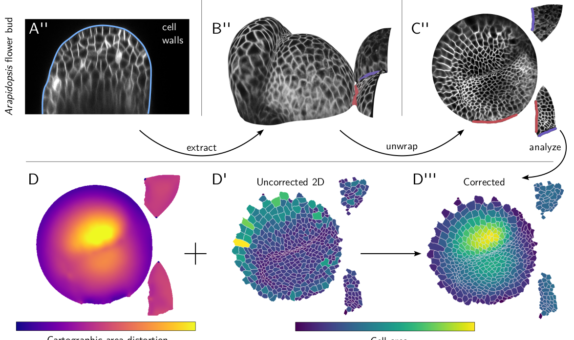
Example: cell segmentation
Here is an example: a volumetric recording of Arabidposis flower buds (shared by Dr. An Yan). After extracting and unwrapping the surface, we can easily segment our cells. But to properly measure the area, we need to take cartographic area distortion into account. We can compute it using diffgeo.get_area_distortion_in_UV. The correct, 3D areas can then be computed using the average distortion factor across each cell.
Vector calculus
For quantitative analysis of changing shapes, one often uses flow or deformation vector fields. For instance, you can use particle image velocimetry, optical flow, or simple cell tracking in 2D projected images to see how cells are moving on top of your 3D surface. Using the diffgeo module, you can map these vector fields from 2D where you computed them back to 3D, and analyze them using the (maybe) familiar tools of vector calculus like \(\nabla\cdot\) and \(\nabla \times\).
Note If your 3D surface is also deforming, you need to add the motion on and the motion of the surface. If you use the reference mesh approach to dynamic data (tutorial 9), it is straightforward to compute the motion of the surface at each position in the 2D projection: just take the difference between the associated 3D coordinates at subsequent timepoints.