Tissue cartography with blender_tisssue_cartography

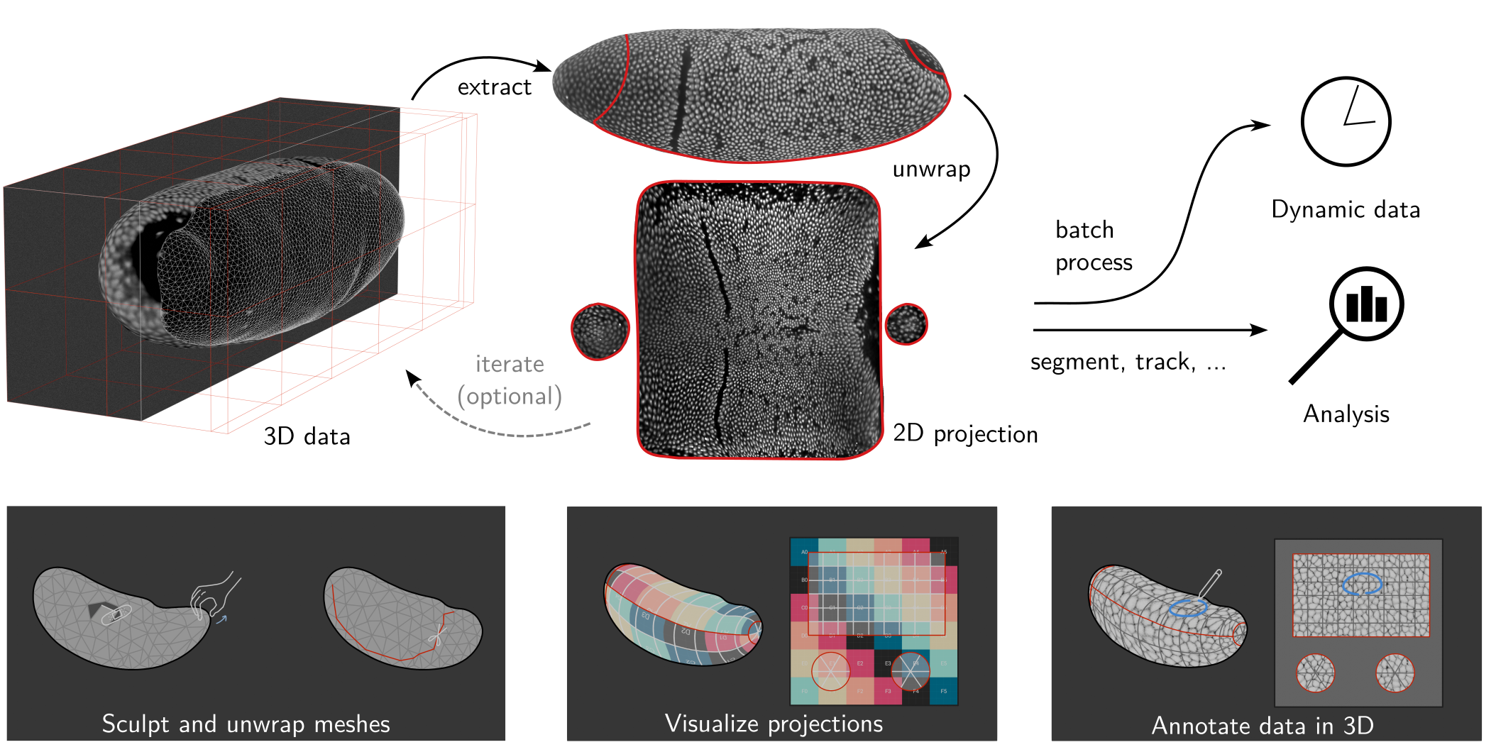
Tissue cartography (TC) is a tool for analyzing 3d biological image data by taking advantage of the laminar, sheet-like organization of many biological tissues. Tissue cartography extracts a surface of interest (SOI) from the volumetric image data, for example, the tube-like structure of the developing fly gut, and cartographically projects it into a 2d plane (see figure below). This is extremely helpful for both data visualization and data analysis, for example cell tracking.

image.png

Tissue cartography was proposed by Heemskerk & Streichan 2015 (ImSAnE software package). See also Mitchell & Cislo 2023 (TubULAR software package) and Herbert et al. 2021 (LocalZProjector software package).

However, these existing tools for tissue cartography are either limited in the type of geometries they can handle, or difficult for non-experts to use and build upon. blender_tisssue_cartography is a set of Python tools, template analysis pipelines, and tutorials to do tissue cartography using the popular 3D creation software Blender. blender_tisssue_cartography makes tissue cartography user-friendly via simple, modular Python code, Blender’s graphical user interface, and powerful algorithms from the computer graphics community.

You can use blender_tissue_cartography in two forms:

1. The blender_tissue_cartography python library

2. The blender_tissue_cartography blender add-on

For sophisticated use cases (dynamic datasets, custom computer vision operation), or automated pipeline, use the python library. Most users though can start with the blender add-on, which allows you to carry out almost all steps of the tissue cartography pipeline within blender’s graphical user interface.

blender_tisssue_cartography also features a general-purpose pipeline for dynamic surfaces from timelapse microscopy in which the user graphically defines a cartographic projection for a single key frame, which is propagated to all other frames via robust surface-to-surface registration algorithms (tutorial 9, “Time-lapse imaging and dynamic surfaces”). A differential geometry module allows to analyze tissue flows and surface geometry dynamics (tutorial 10, “3D analysis and differential geometry”).

Tissue cartography workflow

The TC workflow begins with a volumetric recording, for example, a \(z\)-stack recorded on a confocal microscope. Let’s consider first the case of a single recording with a single time point. TC comprises the following steps:

1. Segmentation: volumetric image \(\mapsto\) 3d segmentation. From the volumetric image - a .tif file , the user creates a 3d segmentation, also a .tif file with values from 0-1. This segmentation divides the image into “inside” and “outside”, and the SOI is defined as the boundary.

   • Note: not all surfaces can be represented as the boundary of a volume. One can also directly segment out the SOI (and use a different algorithm below in step 2).

2. Meshing: 3d segmentation \(\mapsto\) surface mesh. A polygonal mesh of the segmentation boundary is computed, representing the surface of interest.

3. UV mapping: Polygonal mesh \(\mapsto\) cartographic plane. A map from the mesh to a cartographic plane is generated (parametrized by coordinates \(u, v\), to distinguish from the \(x,y,z\) 3d coordinates).

4. Projection: volumetric image + polygonal mesh + UV map \(\mapsto\) projected image. The volumetric image data is interpolated onto the UV cartographic plane using the 3d positions from the triangular mesh, creating a 2d projection of the 3d image data (“pullback”).

   • Multi layers: to capture the whole thickness of a tissue sheet, one typically creates multiple projections using a version of the triangular mesh that is shifted along the local normal direction “inwards” and “outwards”, sort of like peeling an onion.

5. Analysis and visualization: with the projected data in hand, we can visualize it in 3D, or analyse it in 2D (e.g. segment cells), computationally correcting for the distortion of the projection.

6. Batch processing: batch process multiple 3D images, for example frames of a movie.

Tutorials

These steps are explained in detail in our tutorials, which you can find in the website side bar. You can download the tutorial datasets and code from GitHub

1. 3d segmentation with Ilastik. How to segment your data to extract your surface of interest.

2. Blender tutorial How to use the Blender 3D editor and navigate its user interface.

3. blender_tissue_cartography add-on. How to use the btc Blender add-on for tissue cartography (recommended for beginners and for graphically processing new datasets).

4. blender_tissue_cartography Python library How to use the btc Python library(for experts and automated pipelines)

5. Tissue cartography with “seams” How to unwrap complex surfaces using ``seams’’ (cartographic cuts).

6. Iteratively improving cartographic projections How to design the cartographic projection that best fits your data by visualizing the 3D data in Blender.

7. Advanced segmentation and meshing Segmentation and surface extraction for complex and/or “murky” data.

8. Consistent cartographic projections across multiple recordings How to batch-process related datasets so they all use “the same” cartographic projection

9. Time-lapse imaging and dynamic surfaces Tissue cartography for movies.

10. 3D Image analysis with cartographic projections How to use cartographic projections for quantitative analysis and correct for cartographic distortion.

Design principles of blender_tisssue_cartography

1. Blender for graphical, interactive workflows - blender is a widely used, open-source program for 3D creation and contains advanced tools for mesh editing, UV mapping, and 3D visualization within a well-documented GUI. All of the main functionalities are available from within a Blender add-on - no programming knowledge necessary.
2. File-based encapsulation - each step in the pipeline terminates in a single data file (e.g. a .obj mesh, a .tif 3d segmentation), with all subsequent steps only depending on that data file. This means you can easily switch out the tools used for each step.
3. Python library + template Jupyter notebooks. For sophisticated users, the blender_tissue_cartography python library allows creating custom and automatized pipelines. Template / tutorial jupyter notebooks are provided as starting points.
4. UV transfer for dynamic data For dynamic data (i.e. movies), we provide general-purpose algorithms that transfer the user-defined UV map from one frame to all other frames. This allows non-experts to create consistent cartographic projections across time series.

Software stack

• Python libraries:
  • jupyter
  • Numpy / Matplotlib / Scipy
  • skimage various image processing tools.
  • h5py for reading/writing of .h5 files.
  • tifffile for reading/writing of .tif files, including metadata.
  • libigl Triangular meshes.
• Ilastik Image classification and segmentation,
• Blender Mesh editing and UV mapping.

Optional

• Meshlab GUI and Python library with advanced surface reconstruction tools (required for some workflows). Not available for new Macs with ARM CPUs.

• Python libraries:

  • PyMeshLab Python interface to MeshLab. Not available for new Macs with ARM CPUs
  • nbdev for notebook-based development, if you want to add your code

• Blender plugins:

  • MicroscopyNodes for rendering volumetric .tif files in blender

Workflow details

We briefly outline the tools and algorithms available for each step in the tissue cartography pipeline. They are implemented in both the blender_tissue_cartography library, as well as the Blender add-on. This section explains the required input and output data at each step in case you want to swap out the provided tools for something else.

1. Segmentation

To create a segmentation, one first downsamples the data to reduce computational overhead. Next, we can use any of the following tools to create a 3d segmentation:

1. Ilastik - Tutorial 1.
2. Morphsnakes - Tutorial 7
3. Custom Python code

For the segmentation, there are two options:

1. Segment out the object of which your SOI is the boundary (i.e. 1’s in the segmentation correspond to pixels that lie inside the volume of which your surface is the boundary). This assumes that our SOI is a closed/watertight surface (including the case where the SOI ends at the 3d image boundary).
2. Directly segment your SOI (i.e. 1’s in the segmentation correspond to pixels that lie on the surface). See the alternative workflow below. (Generally, option 1 is easier).

Output: 3d segmentation as .tif file

2. Meshing

When the surface is defined as by a volume segmentation (i.e. as a so-called “level set”), robust algorithms exist to compute the corresponding mesh, namely marching cubes and many other.

1. Marching cubes is shipped with blender_tissue_cartography.
2. MeshLab GUI and python library, contains marching cubes and many other tools for surface reconstruction

Alternate workflow: segmentation and meshing for open surfaces

If we have an open surface that is not the boundary of some solid volume, or for some other reason we want to directly segment the surface, we need to use a different algorithm. From our surface segmentation, we extract a cloud of points on the surface. From the point cloud, one can create a triangular mesh using a variety of algorithms, notably Poisson surface reconstruction, as implemented by MeshLab. See tutorial 7.

Output: surface mesh as .obj file

3. UV mapping and mesh processing

To create the map from the mesh to the cartographic \(uv\) plane, we use be blender and its UV mapping functionality. If the mesh looks very poor, we can step back and improve the segmentation and/or meshing. We can also edit the mesh here to correct segmentation/mesh generation errors.

UV mapping conventions

We adopt the UV mapping conventions of the graphics community. \(u,v\) always range from 0-1 (with periodic boundary conditions). In general, blender will always map the entire mesh into the \(u,v\) plane.

Output: surface mesh with normals and texture coordinates as .obj file

4. Projection

Using scipy, we interpolate the volumetric image data onto the \(uv\) plane. Using the vertex normals, we create a multilayer projection.

Output: two .tif \(z\)-stacks (interpolated data and 3d coordinates) and interpolated data as a series of .png images to use as blender textures

5. Visualization and analysis

We can now load the projected data into blender as textures and see whether we are content with the result. If not, we iterate by editing the mesh and/or the \(uv\) mapping. Otherwise, we are done - we can proceed to the analysis of the projected images or use blender to create publication-quality 3d renders.

6. Multiple recordings and movies

If we have multiple recordings of very similar structures or dynamic data, i.e. movies with multiple frames, we need to extract a surface mesh for each timepoint as above. However, we construct a UV map only once, for a suitably chosen keyframe or reference mesh. We then transfer that UV map to all other frames/recordings using surface t0 surface registration algorithms